Motivation

The current paradigm for finding the genetic causes of disease has largely involved Genome-Wide Association Studies (GWAS), which has led to the discovery of thousands of SNPs associated with hundreds of diseases [1, 2, 3, 4]. In a GWAS, researchers aim to identify variants, typically single nucleotide polymorphisms (SNPs), associated with a particular disease or trait by examining the association between genetic variation and the observed phenotype in a large sample of individuals [4]. However, while the scale of GWAS results continues to grow dramatically, the identification of true causal variants or genes associated with traits remains a challenge due to low signal-to-noise ratios and methodological limitations [5]. Further, the great majority of signals in GWAS are located in non-coding regions of the genome, specifically intergenic and intronic regions; this poses a significant challenge for the mechanistic interpretation of GWAS results, as these regions do not code for proteins, and their roles in gene regulation and function are often less well-understood compared to coding regions [6,7]. As we look to gather robust evidence for novel medical and public health interventions, there has been a focus on developing many biological and computational fine-mapping approaches to deduce causal variants in a post-GWAS analysis. This ultimately demands an understanding of the underlying mechanism by which a variant contributes to a trait. Overlapping variants with functional elements, deducing gene regulatory activity, and identifying expression quantitative trait loci (eQTL) are all post-GWAS fine-mapping techniques leveraged for the identification of causal variants associated with a given disease [8, 9].

Here, we explore the use of sensitivity analyses for identifying causal variants from a GWAS. In observational studies like GWAS, the treatment received, namely the genetic variant status in the GWAS context, and disease outcome exhibited may be associated because of some genetic bias, such as linkage disequilibrium (LD), rather than because the variant is actually causally linked to some disease phenotype [10]. Biases visible in measured covariates can be accounted for; however, insensitivity to lurking variables instills more confidence in the findings of an observational study, and skepticism is in fact warranted if only a small degree of hidden bias is required to alter the overall GWAS findings. In particular, with a sensitivity analysis, a GWAS critic cannot necessarily undermine confidence in the significance results by simply stating that hidden bias may exist and instead must specifically argue that the strength of a proposed lurking variable could realistically exceed the maximum degree of bias which a study could absorb while leaving the study’s conclusions intact.

We offer a framework for genetic sensitivity analysis in the context of GWAS, where the assumption of no unmeasured genetic confounders is relaxed gradually. This relaxation is parameterized by a sensitivity value, which depicts the amount of influence we are assuming for the unmeasured confounder, thereby having a useful and intuitive interpretation. We will apply a sensitivity analysis under Rosenbaum’s model [11] since it is both well developed for various observational study structures, and its properties have been well studied. Marginally, by variant, we seek to estimate the maximum degree of bias or confounding that can be introduced such that the results remain significant, and we discuss the potential for applying a joint sensitivity analyses to aggregate results (e.g. to the gene level). In this framework, we can gain insight into the causality of each variant for a given disease outcome or trait; it is hypothesized that each variant’s estimated sensitivity value will provide utility in inferring its level of causality for a given trait or disease outcome.

We first provide a detailed derivation of the sensitivity model in a general causal inference context, and we demonstrate its utility in a “simple case” simulation. We subsequently simulate a genetic architecture and disease phenotype, and we tailor this sensitivity to our simulated genetic context. Note that scaling the sensitivity analysis framework for the analysis of millions of genetic variants is a challenge of this method, which we strategically address using a variety of statistical and computational techniques. The application of this method beyond simulation studies, perhaps to Biobank scale data, is an exciting next step of this proposed work.

We argue for the inclusion of such post-GWAS sensitivity analyses for more robust insights generation. By integrating sensitivity analysis into the GWAS framework, we aim to provide a novel approach for identifying causal variants related to disease outcomes and traits, ultimately contributing to a deeper understanding of the genetic basis of complex diseases.

General Sensitivity Analysis

Sensitivity analysis is a powerful technique commonly used in various fields, such as economics, engineering, and environmental sciences, to assess the robustness of statistical conclusions. In observational studies, sensitivity analyses allow a researcher to explore the potential impact of hidden biases or unmeasured confounders on the conclusions of a study. In particular, the goal of a sensitivity analysis is to evaluate the stability of the observed associations and provide a quantification of the uncertainty or potential bias in the results.

Setup

Consider an observational study with \(N\) total individuals placed into \(I\) matched sets by an optimal without-replacement matching algorithm. Let \(n_i\) represent the number of individuals in the \(i\)th matched set, and let \(W_ij\) be the binary treatment indicator for the \(j\) individual in the \(i\)th matched set; we assume that the \(i\)th matched set is comprised of only 1 treated individual and \(n_i-1\) control individuals such that \(\sum_{j=1}^{n_i} W_{ij} = 1\). Also let \(y_{1ij}\) and \(y_{0ij} =\) potential outcome for the \(ij\)th individual under treatment and control, respectively. Also, let \(\mathbf{x}_{ij}\) and \(u_{ij}\) denote the observed covariates and unobserved covariates for this \(ij\)th individual. Finally, let \(\mathcal{F} = \{(y_{0ij}, y_{1ij}, \mathbf{x}_{ij}, u_{ij}): i = 1,\dots,I; j = 1,\dots, n_i\}\) be the set containing all aforementioned objects across all individuals and matched sets in the study.

In a population, we assume that individuals receive treatment independently; let \(\pi_{ij} = \text{Pr}(W_{ij} = 1\\|y_{0ij}, y_{1ij}, \mathbf{x}_{ij}, u_{ij})\) be the probability that \(ij\)th individual received treatment. We can then write,

Note that \(\mathbf{W} = (W_{11}, W_{12}, \dots, W_{n_11}, W_{21}, \dots, W_{In_I})^\top\) is a lexicographically ordered vector of treatment assignments, and we henceforth adopt similar notation for other boldfaced variables. Note that in a sensitivity analysis, we assume that treatment assignment is strongly ignorable given both the observed and unobserved covariates \((\mathbf{x}, u)\), not simply the observed covariates.

Rosenbaum and Krieger [11] introduce the following sensitivity analysis model. Consider bounding the ratio of odds ratios of \(\pi_{ij}\) and \(\pi_{ik}\) for two individuals \(j,k\) in the same matched set \(i\),

\begin{equation} \frac{1}{\Gamma} \leq \frac{\frac{\pi_{ij}}{1-\pi_{ij}}}{\frac{\pi_{ik}}{1-\pi_{ik}}} = \frac{\pi_{ij}(1-\pi_{ik})}{\pi_{ik}(1-\pi_{ij})} \leq \Gamma, \qquad \text{for } i = 1,\dots, I; j,k = 1,\dots, n_i \end{equation}

The key idea behind a sensitivity analysis is that hidden bias exists if two units with the same, or similar, covariates have different chances of receiving treatment. To see this more explicitly, recognize that at \(\Gamma = 1\), two individuals in the same matched set, namely matched on their observed covariates, have the same probability of receiving treatment. We can then equivalently see that at this \(\Gamma=1\) value, \(\text{Pr}(W_{ij} = 1 \\| y_{0ij}, y_{1ij}, \mathbf{x}_{ij}, u_{ij}) = \text{Pr}(W_{ij} = 1 \\|\mathbf{x}_{ij})\), indicating that a study is free of hidden bias or unmeasured confounders. In other words, at \(\Gamma = 1\), matching generates a reference distribution for estimating treatment effects that corresponds to the distribution we would have achieved via controlled experimentation. Taking \(\Gamma > 1\) quantifies deviations from equal assignment probabilities within a matched set, where larger values of \(\Gamma\) indicate more hidden bias or unmeasured confounding.

Propensity Score Matching

A critical step in this sensitivity analysis framework is the construction of \(I\) matched sets, within which the observed covariates are balanced. Here, we leverage the propensity score, proposed by Rosenbaum and Rubin [12]; the propensity score is the conditional probability of assignment to treatment given the set of observed covariates, \(\text{Pr}(W_{ij} = 1 \\| \mathbf{x}_{ij})\). Adjustment for the scalar propensity score is sufficient to remove bias due to all observed covariates; specifically, Rosenbaum and Rubin [12] show that matching on the propensity score tends to balance the observed covariates used to estimate this score, and likewise, for balancing these observed covariates, it suffices to balance the one-dimensional propensity score.

The propensity scores are estimated by regressing the treatment assignment on the set of observed covariates that we want to balance. Individuals can subsequently be matched based on their propensity scores by nearest neighbor matching [13]. Generally, in this “greedy” algorithm, each treated individual is matched to the set of control individuals with the closest propensity scores sequentially to form the matched sets. In this study’s setup, to accommodate a varying number of control individuals in each matched set, namely depending on the availability of control data, we perform nearest matching as follows. All individuals are first sorted in a vector based on propensity score. We then walk along this vector, collecting control individuals; when a treated individual is reached, all collected individuals and half of the control individuals before the next treated individual are assigned to the given treated individual’s matched set. In the case of subsequent treated individuals in this sorted propensity score vector, the nearest control individual available is simply assigned to a matched set, such that every matched set has at least one control individual.

Note that this sequential matching strategy does not necessarily achieve the global matching optimum, which we assumed for convenience in the sensitivity analysis model. However, it does achieve nearly linear time complexity, which is a particularly important condition once we scale the sensitivity analysis model for millions of variants in the genome-wide application.

Constructing Bounds on Association p-values

In a sensitivity analysis, recall that the general strategy is to find the maximum degree of bias or confounding that can be introduced such that a study’s results remain significant. Accordingly, we proceed by constructing bounds on the \(p\)-value with respect to a given test statistic, assuming that the sensitivity model (1) holds at a given value \(\Gamma\). In particular, we want to find the worst-case \(p\)-value assuming the sensitivity model (1) holds at some value \(\Gamma\); denote this \(p_\Gamma\). The given value \(\Gamma\geq 1\) is then increased gradually until the worst-case upper bound on the \(p\)-value exceeds a specified significance level \(\alpha\); we are particularly interested in the smallest \(\Gamma\) for which \(p_\Gamma > \alpha\), which is referred to as the “sensitivity value”.

Importantly, this sensitivity value provides a measure of robustness for our significance result as it necessarily describes the minimum degree of bias required to render or results non-significant. Insensitivity to a large degree of hidden bias, represented by a large sensitivity value, provides confidence in the conclusions of an observational study; on the other hand, if only a small degree of hidden bias is required to render our conclusions nonsignificant, skepticism might in fact be warranted.

Here, we assume a particular form of test statistics. In general, first let \(G(\mathbf W, \mathbf Y)\) be an arbitrary function of both the vector of treatment assignments \(\mathbf W\) and the vector of observed outcomes \(\mathbf Y\). For any vector of unmeasured confounders \(\mathbf u \in \mathcal{U}\), where \(\mathcal{U}\) is the \(N\)-dimensional unit cube, when the sensitivity analysis model (1) is assumed to hold at a given \(\Gamma\), [14] show that the randomization distribution of \(G(\mathbf W, \mathbf Y)\) takes the form

where \(\Omega\) is the set of treatment assignments \(\mathbf w\) adhering to the matched design, namely satisfying \(\sum_{i=1}^{n_i} w_{ij} = 1\) for all \(i\). Now, consider a scalar-valued test statistic \(T(\mathbf W, \mathbf F)\), where \(F_{ij} = W_{ij} f_{1ij}(y_{1ij}) + (1-W_{ij})f_{0ij}(y_{0ij})\) and \(f\) is simply a function of the potential outcomes; suppose that larger values for the test statistic reflect evidence against a sharp null hypothesis. The right tail probability for \(T(\mathbf W, \mathbf F)\) under the sharp null hypothesis is then \begin{equation} \text{Pr}\left{T(\mathbf W, \mathbf F) \geq t | \mathcal{F,W}, \mathcal{H}{sharp}\right} = \frac{\sum{b\in\Omega} \exp(\gamma \mathbf b ^\top \mathbf{u}) 1{T(\mathbf b , \mathbf F) \geq t}}{\sum_{b\in\Omega}\exp(\gamma \mathbf b ^\top \mathbf{u})} \end{equation}

More specifically here, we consider test statistics of the form \(T(\mathbf W, \mathbf F) = \mathbf W ^ \top \mathbf q\), for some vector \(\mathbf{q} = \mathbf{q}(\mathbf F)\), which is referred to as the sum statistic; most widely-used test statistics can actually be adapted to this form. We can construct random variables \(T_\Gamma^-\) and \(T_\Gamma^+\) whose upper tail probabilities bound the upper tail probabilities in (2) for any \(t\) at a given value of \(\Gamma\). Namely, we want to construct these random variables such that

where \(t_0\) is the observed value of the test statistic in the study. While the lower bound on the right-tail probability of a test statistic may be of interest in some contexts, here, we focus on finding the distribution of the upper bound from the random variable \(T^+_\Gamma\).

We can easily construct these bounding random variables for simple sign-score sum statistics; however, for other sum statistics after matching for multiple controls, it becomes computationally intractable to apply this bounding procedure and optimize over the \(\prod_{i=1}^I(n_i-1)\) elements of \(\mathcal{U}^-\) and \(\mathcal{U}^+\) [15]. As a result, Stuart and Hanna [16] leveraged an asymptotic approximation on termed asymptotic separability. This approach is based on a Normal approximation for the distribution of \(\mathbf W ^ \top \mathbf q\). When the sensitivity model (1) is assumed to hold at \(\Gamma\), we can construct a Normal random variable \(\tilde T^+_\Gamma\) whose moments we can derive. The general strategy is to find the vector \(\mathbf u\), which maximizes the expected value of \(\mathbf W ^ \top \mathbf q \\| \mathcal{F, W}\) when the sensitivity model holds at \(\Gamma\); we then compute the relevant right tail probability for a Normal random variable with the this maximal expectation and variance. What makes this approach particularly advantageous is the fact that the mean and variance may be pieced together separately within each matched, requiring optimization over only \(n_i-1\) candidate solutions for each matched set \(i\) rather than global optimization.

To derive the mean and variance of \(\tilde T_\Gamma^+\), we first rearrange the values \(q_{ij}\) in each matched set \(i\) such that \(q_{i1} \leq q_{i2} \leq \cdots \leq q_{in_i}\). Let \(\mathcal{U}_i^+\) denote the collection of \(n_i-1\) binary vectors for the \(i\)th matched set of the form \(u_{i1} = \cdots = u_{ia_i} = 0\) and \(u_{ia_i+1} = \cdots = u_{in_i} = 1\) for some \(a_i = 1, \dots, n_i - 1\). We can first find \(\mu_i^+\), the largest possible expectation for \(\mathbf u_i \in \mathcal{U}_i^+\),

where \(\gamma = \log \Gamma\). Likewise, we can find \(\nu_i^+\), the corresponding maximal variance,

where \(\mathcal{A}_i\) is the set of \(a_i\) attaining the maximal expectation \(\mu_i^+\), in the case of potential ties for the maximum expectation. Then, by independence of conditional treatment assignments across matched sets, the expectation and variance of the asymptotic bounding Normal random variable \(\tilde T_\Gamma^+\) as

And thus, the asymptotic upper bound for \(\text{Pr}(\mathbf W ^\top \mathbf q \geq t_0 \\|\mathcal{F}, \mathcal{W})\) from this asymptotic bounding procedure is,

where \(\Phi\) is the cumulative density function of the standard Normal distribution. Note the procedure for finding the moments of \(\tilde T_\Gamma^-\) is directly analogous, only requiring that we replace \(q_{ij}\) with \(\tilde q_{ij} = - q_{ij}\) for all \(ij\) in the above derivations; however, this lower bound on the tail probability is not necessarily of interest for the applications here.

Simple Case Simulation

Before applying this sensitivity analysis for deducing causal variants from a GWAS, we first demonstrate the utility of the method in detecting unobserved covariates or hidden bias in a simple case simulation. In particular, we show that a sensitivity value is a more robust measure for the detection of unobserved bias or confounding in a study design, as opposed to simply relying on an association \(p\)-value.

For \(N=1000\) individuals, we start by simulating observed covariates \(x_i \overset{iid}{\sim}\mathcal{N}(0,1)\) and unobserved covariates \(u_i \overset{iid}{\sim} \mathcal{N}(0, \sigma^2_u)\), where the unobserved effect is parameterized through \(\sigma^2_u\). We then assign each individual a probability of receiving treatment based on the observed and unobserved covariates; the \(i\)th individual’s propensity score \(p_i\) is simulated according to

Potential outcomes \(y_{0i}\) and \(y_{1i}\) can subsequently be simulated according to, \(y_{i0} = x_i + u_i + \epsilon_i\) and \(y_{i1} = x_i + u_i + \tau + \epsilon_i\), where \(\epsilon_{ij}\sim\mathcal{N}(0,1)\) and \(\tau\) is the treatment effect; here, we use \(\tau = 2\).

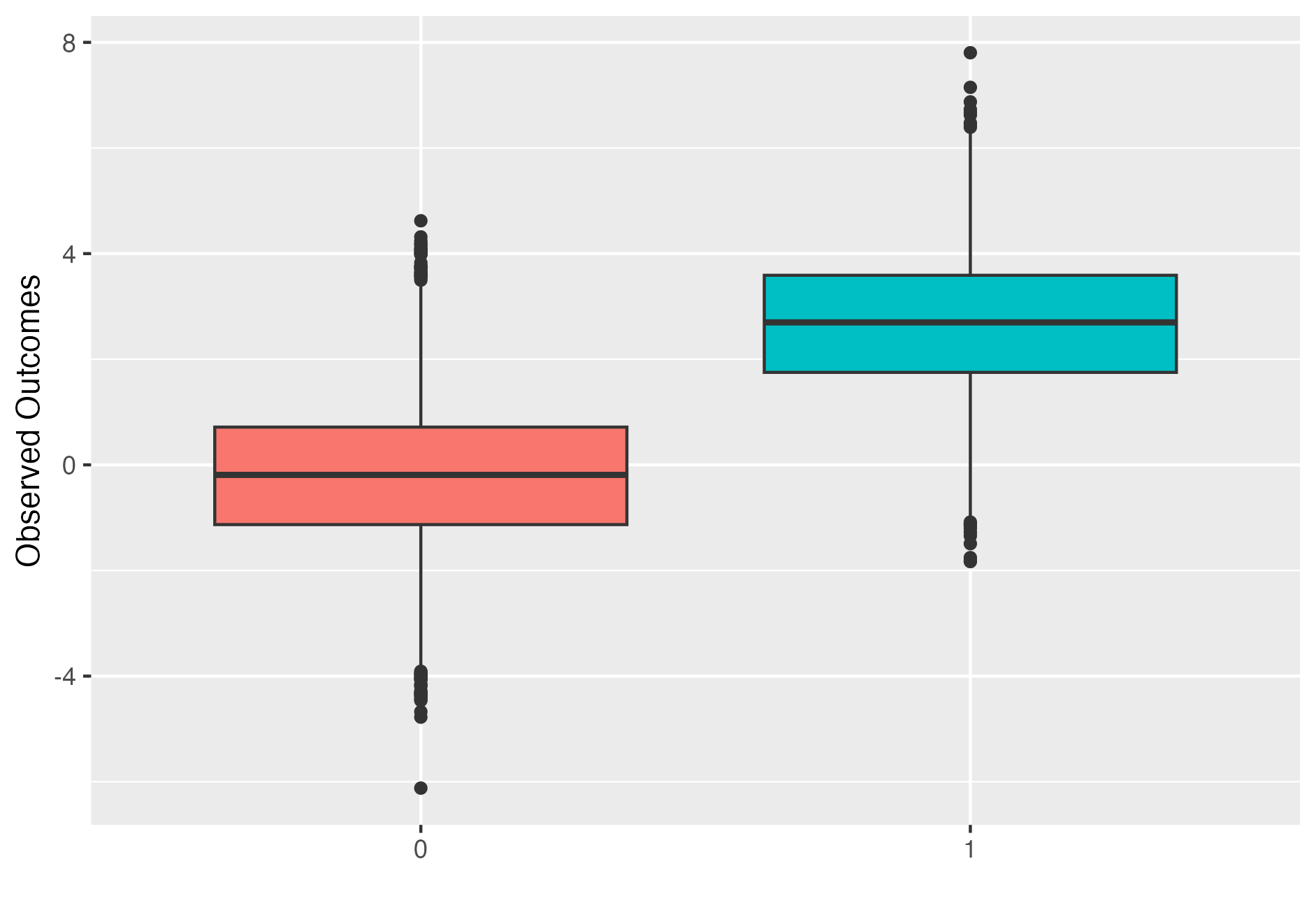
Simulated observed outcomes for \(N=1000\) individuals and a treatment effect of \(\tau=2\). Treated individual outcome are represented by right box plot.

To run the sensitivity analysis, we begin by estimating propensity scores for all individuals, shown in the figure below, and using these scores to match individuals. In this simple case simulation, we use a paired setting where each matched set contains a treatment-control pair. As a result, we apply a Wilcoxon rank sums test to conduct this sensitivity analysis.

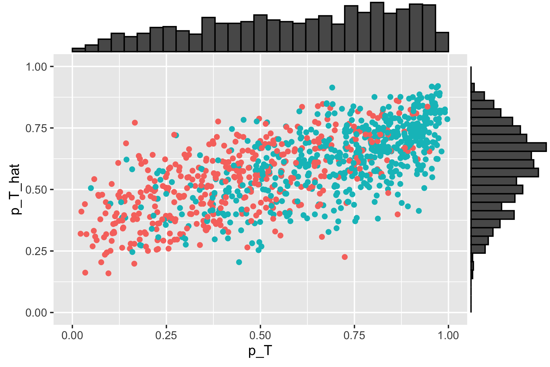
Scatterplot of true versus estimated propensity scores with \(\sigma_u^2 = 1.5\). True simulated propensity values are included on the horizontal axis, and estimated propensity scores are included on the vertical axis.

With this simple case data simulated, we can test the sensitivity analysis model at different levels of hidden bias or confounding. Specifically, we test \(\sigma_u^2 = \{0.5, 0.6, \cdots, 4\}\) values, running both a sensitivity analysis and a regression in each case. Below, we show the results from this simulation testing procedure.

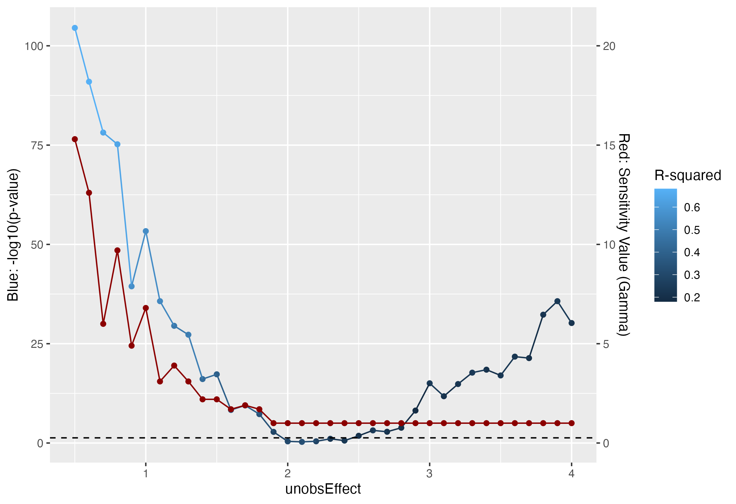
Results from association tests and sensitivity analysis across several values of \(\sigma^2_u = 0.5, \dots, 4.0\). Red points represents sensitivity values, namely the minimum \(\Gamma\) such that \(p_\Gamma > \alpha\), and the blue points represent the association \(p\)-values, on a \(-\log10\) scale, calculated by regressing the outcomes on the treatment assignment. Horizontal dashed line represents the typical \(\alpha = 0.05\) significance threshold. Sensitivity values appear more stable as the unobserved effect increases, and evidence of unobserved effects is quickly detected around \(\sigma^2_u = 1\). On the other hand, regression produces significant treatment effect until \(\sigma^2_u = 2\).

We see from the figure above that sensitivity values do in fact provide robust measure of the degree of bias or unobserved covariates than simply relying on the results from a simple regression. As expected, the sensitivity value drops as the unobserved confounding effect, namely \(\sigma^2_u\), increases; we have fairly strong evidence of unobserved confounding effects around \(\sigma^2_u = 1\). Simply relying on an association \(p\)-value, we would have evidence of unobserved confounding until \(\sigma^2_u = 2\), when the unobserved covariate already has double the variance of the observed covariate. We do see that the \(R^2\) value decreases with increased unobserved effects. However, it is important to remember that we simulate only two covariates in this case, one of which is unobserved; in this case, it is easy to interpret the \(R^2\) value and assume that any decrease in \(R^2\) is attributable to an unobserved covariate. In a realistic setting, further estimation procedures would be needed to make inferences on the observed \(R^2\) value.

Genomic Sensitivity Analysis

With the foundation and sensitivity model framework outlined, we tailor this approach for the GWAS context, with the goal of identifying causal variants from genomic data. Note that the theoretical adaptations of the sensitivity model are minimal, yet perhaps the most challenging obstacle ahead of this goal is maintaining reasonable computational resources and runtime when running this analysis genome-wide. We discuss some key strategies taken to overcome this obstacle and apply our method on simulated genomic data to demonstrate its utility.

GWAS Sensitivity Model Framework

In the most basic form of GWAS, the outcome, namely a trait or disease phenotype, is regressed marginally on each variant’s dosage to estimate both the variant effect size and the association \(p\)-value. While this approach has shown success in identifying variants of large effects, it remains difficult to identify causal variants in LD blocks (represented by “towers” on GWAS Manhattan plots), and association does not typically translate to causality in the genomic setting.

Here, we propose using the sensitivity analysis model to deduce causal variants from a GWAS. Consider a single SNP in a GWAS of \(N\) individuals, specifically, the \(N\)-dimensional dosage vector. We can treat allele dosage as the treatment assignment to conduct our sensitivity analysis, essentially asking if there is hidden bias or unobserved confounding beyond the given SNP dosage which would bias or overturn the association conclusions observed in our study. Similar to before, insensitivity to strong confounding, as evidenced by a high sensitivity value, instills confidence in the association conclusion made and perhaps even suggests causality.

Treating each SNP as the treatment assignment in a given observational study, we intuitively seek to arrive at a test statistic which capture the “per-allele” mean difference in outcome as an estimate for the treatment effect. We can thus reasonably construct a test statistic of the following form,

where the \(it\) individual refers to the one treated individual in each matched set. In this case, we see that our particular sum statistic \(q_{ij} = \sum_{j'=1}^{n_i} (y_{ij} - y_{ij'})/(I(n_i - 1))\) gives us the treated minus control difference in means within each matched set. Note that the absolute value of the test statistic was considered in this case since treatment effect can potentially be negative (e.g. for deleterious variants), adjusting probabilities in the previous derivations as necessary.

For matching, individuals with one or two copies of the effect allele were typically considered treated individuals; in cases where the number of one- or two-copy individuals exceeded the controls, one-copy individuals were considered control to proceed with matching. The effects of this decision on the sensitivity values calculated are discussed in a later section. With the appropriate test statistic defined, we can proceed by running the sensitivity analysis model described in the earlier section, in particular leveraging the idea of asymptotic separability to upper bound the right tail probability of interest.

Computational Efficiency Genome-Wide

When scaling the sensitivity model described here to the genome-wide level, computational resource and time efficiency become important considerations or obstacles that must be addressed to make the method applicable and widely available. From a methodological standpoint, we have already implemented a few approaches to make this sensitivity model efficient, such as the asymptotic separability assumption [16] and the decision to use propensity score matching instead of optimal matching. Matching was perhaps the biggest hurdle that had to be overcome to apply the sensitivity analysis genome-wide, and reducing this step to linear time complexity, albeit forgoing optimality, was critical.

Computationally, we also applied several strategies to make this strategy computationally feasible and efficient. Genotype matrices are large files that can be difficult to store or repeatedly access. Here, we stored genotype matrices in binary format to keep the file sizes manageable. We leveraged several programs, such as plink [17] and GCTA [18] to operate on these binary matrices and avoided reading in the full matrix into memory at once; specific elements of this matrix were read into memory as needed and subsequently freed to keep the computational resources needed to run the sensitivity analysis minimal.

Multi-threading and parallel computing were also leveraged to speed up the genome-wide sensitivity analysis. In particular the “parallel” library in R was used. Since sensitivity analyses are run marginally for each variant, multiple analyses can simply be run in parallel to reduce the time needed to complete the genome-wide sensitivity analysis.

Simulation of Genetic Data

We explore the utility of the sensitivity model in a genome-wide context via simulation. Genetic simulations were performed using real genetic data from the HapMap cohort, thereby maintaining existing LD patterns in such cohorts; here we test \(N = 15000\) individuals. Disease phenotypes were then simulated as linear combinations of dosage weighted by simulated SNP effects. Hertiability, the proportion of phenotypic variance explained by all measured SNPs, was fixed at 40%, and SNP effects were simulated using the GCTA software [18]. To explore performance across varying genetic architectures, we considered two cases. Case 1 represented a disease where 0.01% of SNPs, namely 117 SNPs, across the genome were causal, and case 2 represented a disease where 25% of SNPs, namely 293,720 SNPs, across the genome were causal. Causal SNP effects were simulated from a Normal, and all other SNPs had an true effect of exactly zero. Note that since heritability is fixed at 40%, case 1 consisted of fewer SNPs of considerably higher effects, whereas case 2 consisted of many more SNPs of very low effect sizes.

We then simulated non-genetic covariates for matching, including age, which was Uniformly distributed from 20 to 80, sex, which was a binary trait, and another Normally distributed covariate, centered at 22 with a variance of 4 (e.g. BMI). Then, to simulate a non-genetic component for the overall the phenotype, we simply calculated a weighted sum across the covariates \(\sum_{k=1}^P \beta_k C_{ijk}\) where the \(\beta_k\) covariate effects were fixed (ranging from 0.3 to 0.9), \(P\) is the number of simulated covariates, and \(C_{ijk}\) is the value of the \(k\)th covariate for the \(ij\)th individual. Non-genetic effects were then scaled and added to the simulated genetic component of the phenotype to arrive at the overall observed phenotype for each individual.

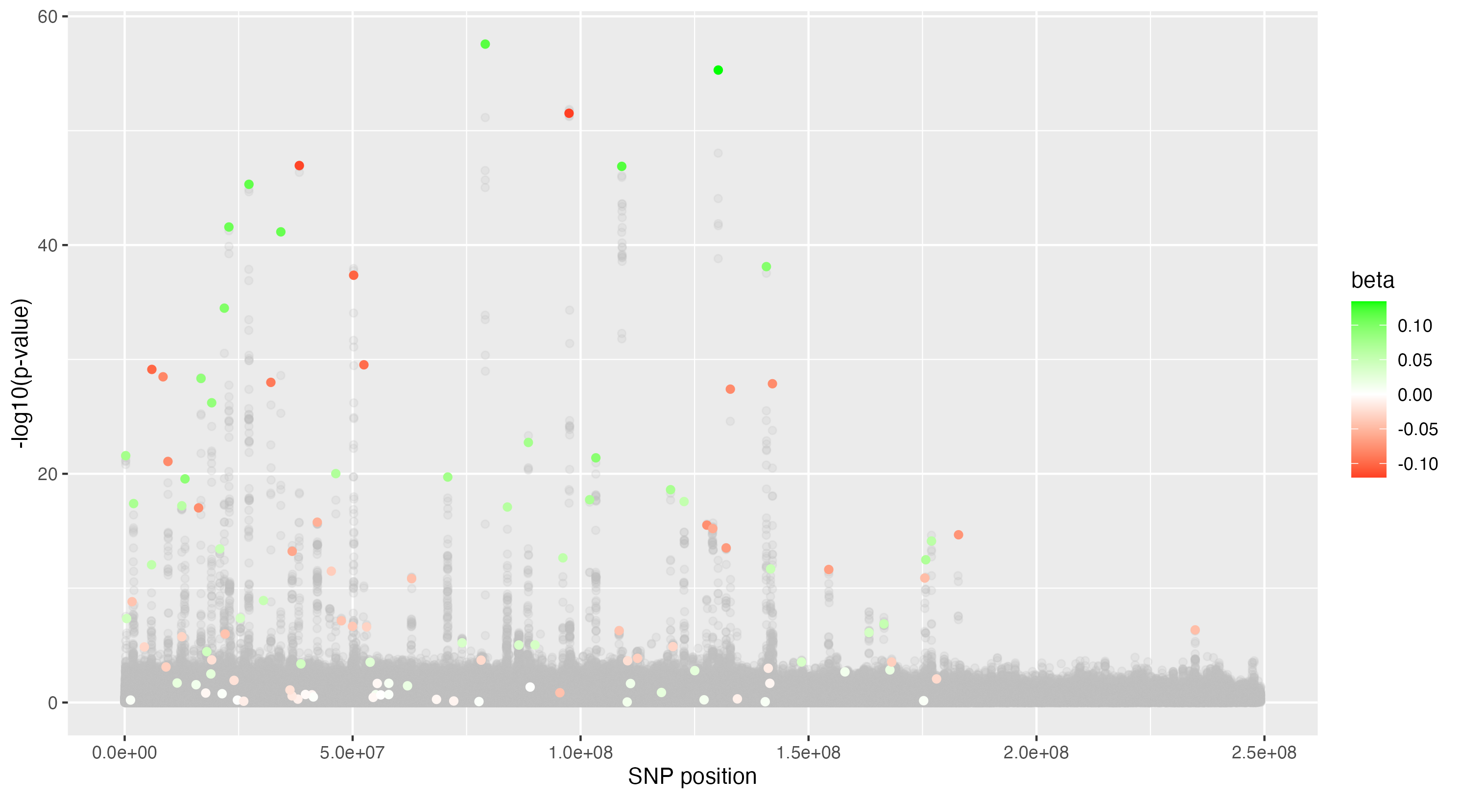
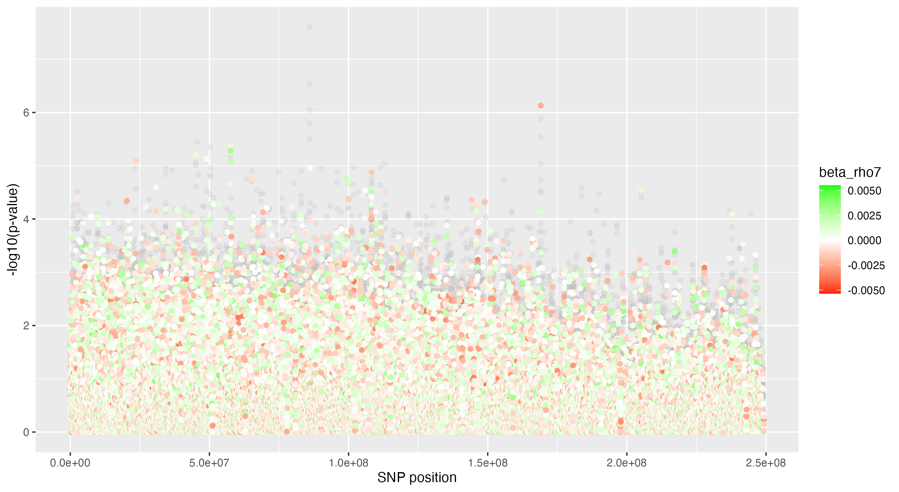
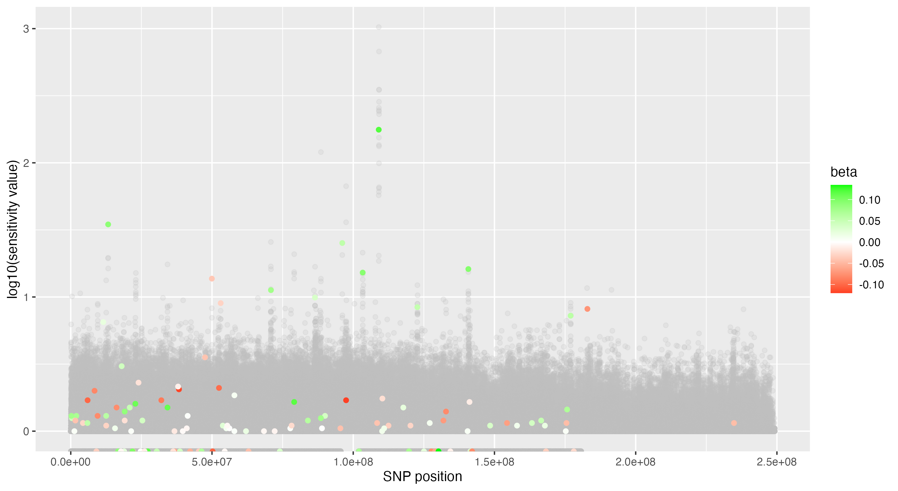
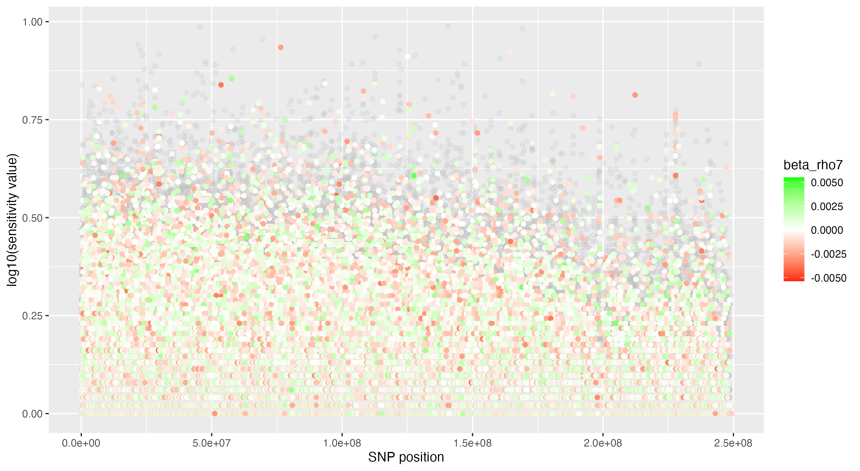
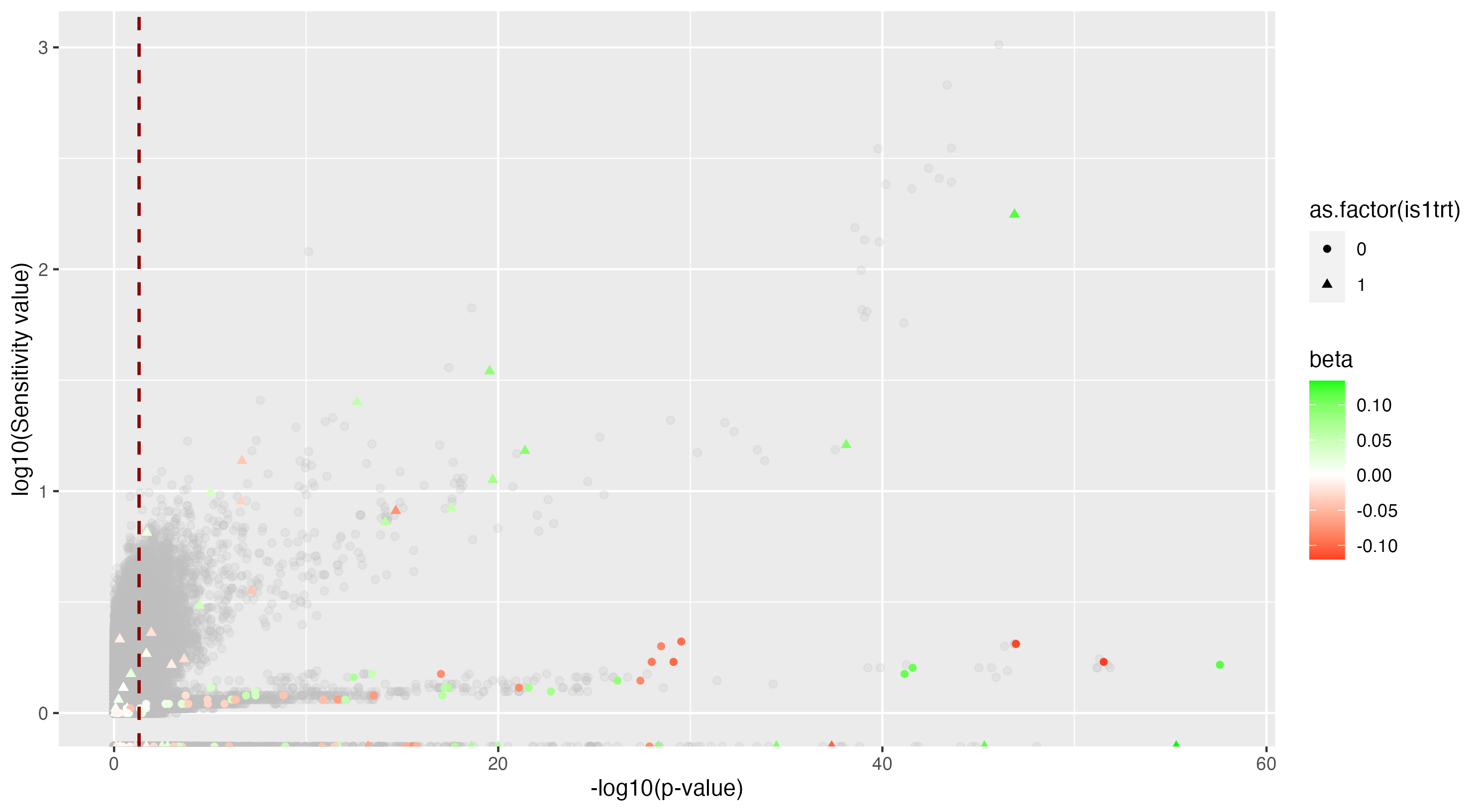
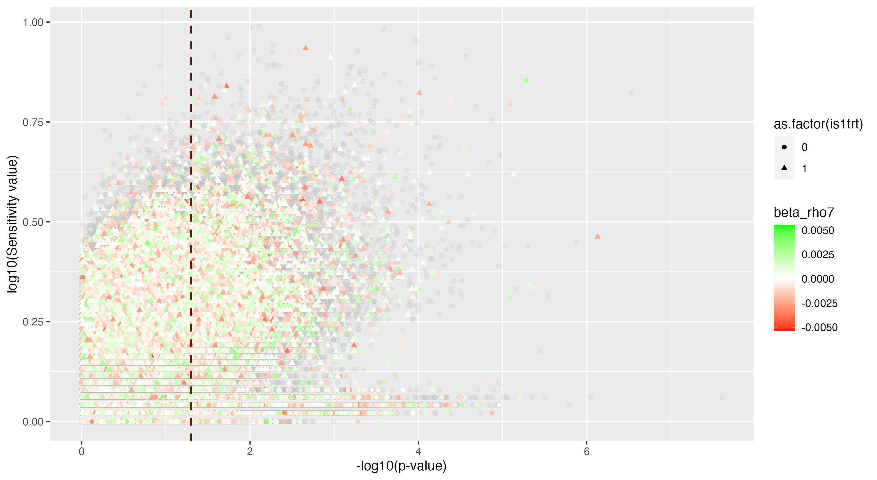
We then proceeded by running the sensitivity analysis genome-wide; results are included in figures below. Results from case 1 with 0.01% causal SNPs are included in the left column, and results from case 2 with 25% causal SNPs are included in the right column.

(a)

(b)

(c)

(d)

(e)

(f)

We see that in case 1 with few high-effect casual SNPs, a GWAS analysis is able to effectively detect SNPs of high effects, as shown by the Manhattan plot in (a); such SNPs are typically found at the top of their LD towers. On the other hand, the sensitivity analysis is not necessarily as effective at identifying the causal variants. Non-causal variants often receive high sensitivity values, and several causal variants receive relatively low sensitivity values.

However, in (e), we find a potential explanation for these results. By plotting the sensitivity values against the association \(p\)-values, we do find general concordance across the two methods; however, recall that if the proportion of one- and two-copy individuals exceeded the number of zero-copy individuals, the matching procedure was adapted such that one-copy individuals were treated as controls, adjusting the test statistic accordingly. We find that in cases where the one-copy individuals were treated as control individuals, sensitivity values tended to be deflated, thereby leading to several false negatives. This suggests that perhaps a modified test statistic or alternative matching procedure must be developed to deal with variants with high proportions of heterozygotes, namely individuals with one-copy of the variant allele. These patterns are largely maintained in the case 2 genetic architecture though perhaps here.

Discussion

In this work, we apply the sensitivity model framework to a GWAS context to identify causal variants genome-wide. Through a simple case simulation and a genetic simulation, we evaluated the utility of this method in identifying sources of hidden bias or unobserved confounders. There were certainly shortcoming and challenges faced when applying this method genome-wide. In the genetic simulation, we found that the sensitivity values estimated were not always highest for causal variants of nonzero effects. For some of these variants, deflated sensitivity values may be due to the fact that one-copy individuals were used as control individuals in the matching procedure. Nevertheless, generally, these findings suggest that there is room for this sensitivity analysis procedure to be further developed and adapted to this genomic context.

In the case of a GWAS, a variety of approaches are used to deduce causal variants, from clumping to fine-tuning. LD blocks, namely regions where SNPs are inherited together due to infrequent genetic recombination, complicate this causality inference; SNPs surrounding a truly causal SNP may be flagged as significant only due to these LD patterns. Rather than inferring this LD through a sensitivity analysis as we implicitly sought to do here, a potentially fruitful extension of this work is to directly model surrounding SNPs as observed covariates to be adjusted for by matching. In other words, by matching based on proximal SNPs (e.g. via propensity score matching), LD patterns can potentially be controlled for and a truly causal SNPs may be easier inferred as a result. In fact, the ignorability assumptions necessary when SNP dosage is used as treatment may be more valid in this framework.

Perhaps another concern of the approach applied here is the decision to use SNP dosage directly in the test statistic. Typically, genotypes are standardized in a GWAS to control for factors such as allele frequency and population stratification, and we can explore similar standardization procedures to produce more robust and meaningful test statistics. Note that the performance of a sensitivity analysis model here is greatly influenced by the choice of test statistic, so perhaps more robust test statistics tailored to the distribution of the underlying genetic architecture, or the presence of gene-environment interactions may produce some novel insights.

It is important to note that here, we compare our model to the most standard form of GWAS, but a plethora of methods have been introduced to address the shortcomings of a standard regression-based approach. In particular, Bayesian shrinkage-based methods such as Lassosum [19] and REGENIE [20] have been introduced to deduce causal variant signals from noise across the genome, and these approaches have shown great success in some cases. In this work, we do compare to a marginal form of GWAS though since the sensitivity analysis model is similarly applied marginally.

Ultimately, the method introduced here does provide researchers with an important level of insight that is typically missed in conventional GWAS. By running a sensitivity analysis, researchers can critically assess the robustness of their findings and directly estimate the potential influence of unmeasured confounders on their observed associations. This can help to mitigate the impact of hidden biases and improve the validity of the results, leading to more reliable inferences about the causal relationship between genetic variants and disease outcomes.

References

[1] S. E. Bergen and T. L. Petryshen. Genome-wide association studies of schizophrenia: does bigger lead to better results? Current opinion in psychiatry, 25(2):76–82, 2012.

[2] L. Bertram and R. E. Tanzi. Genome-wide association studies in alzheimer’s disease. Human molecular genetics, 18(R2):R137–R145, 2009.

[3] B. P. Prins, V. Lagou, F. W. Asselbergs, H. Snieder, and J. Fu. Genetics of coronary artery disease: genome-wide association studies and beyond. Atherosclerosis, 225(1):1–10, 2012.

[4] E. Uffelmann, Q. Q. Huang, N. S. Munung, J. De Vries, Y. Okada, A. R. Martin, H. C. Martin, T. Lappalainen, and D. Posthuma. Genome-wide association studies. Nature Reviews Methods Primers, 1(1):59, 2021.

[5] V. M. Walker, J. Zheng, T. R. Gaunt, and G. D. Smith. Phenotypic causal inference using genome-wide association study data: Mendelian randomization and beyond. Annual review of biomedical data science, 5:1–17, 2022.

[6] M. J. Li, P. Wang, X. Liu, E. L. Lim, Z. Wang, M. Yeager, M. P. Wong, P. C. Sham, S. J. Chanock, and J. Wang. Gwasdb: a database for human genetic variants identified by genome-wide association studies. Nucleic acids research, 40(D1):D1047–D1054, 2012.

[7] D. Welter, J. MacArthur, J. Morales, T. Burdett, P. Hall, H. Junkins, A. Klemm, P. Flicek, T. Manolio, L. Hindorff, et al. The nhgri gwas catalog, a curated resource of snp-trait associations. Nucleic acids research, 42(D1):D1001–D1006, 2014.

[8] B. Zeng, J. Bendl, R. Kosoy, J. F. Fullard, G. E. Hoffman, and P. Roussos. Multi-ancestry eqtl meta-analysis of human brain identifies candidate causal variants for brain-related traits. Nature genetics, 54(2):161–169, 2022.

[9] K. Wang, M. Li, and H. Hakonarson. Annovar: functional annotation of genetic variants from high-throughput sequencing data. Nucleic acids research, 38(16):e164–e164, 2010.

[10] M. Slatkin. Linkage disequilibrium—understanding the evolutionary past and mapping the medical future. Nature Reviews Genetics, 9(6):477–485, 2008.

[11] P. R. Rosenbaum and A. M. Krieger. Sensitivity of two-sample permutation inferences in observational studies. Journal of the American Statistical Association, 85(410):493–498, 1990.

[12] P. R. Rosenbaum and D. B. Rubin. The central role of the propensity score in observational studies for causal effects. Biometrika, 70(1):41–55, 1983.

[13] P. C. Austin. A comparison of 12 algorithms for matching on the propensity score. Statistics in medicine, 33(6):1057–1069, 2014.

[14] J. R. Zubizarreta, E. A. Stuart, D. S. Small, and P. R. Rosenbaum. Handbook of Matching and Weighting Adjustments for Causal Inference. CRC Press, 2023.

[15] P. R. Rosenbaum. Impact of multiple matched controls on design sensitivity in observa- tional studies. Biometrics, 69(1):118–127, 2013.

[16] E. A. Stuart and D. B. Hanna. Commentary: Should epidemiologists be more sensitive to design sensitivity? Epidemiology, 24(1):88–89, 2013.

[17] S. Purcell, B. Neale, K. Todd-Brown, L. Thomas, M. A. Ferreira, D. Bender, J. Maller, P. Sklar, P. I. De Bakker, M. J. Daly, et al. Plink: a tool set for whole-genome associ- ation and population-based linkage analyses. The American journal of human genetics, 81(3):559–575, 2007.

[18] J. Yang, S. H. Lee, M. E. Goddard, and P. M. Visscher. Gcta: a tool for genome-wide complex trait analysis. The American Journal of Human Genetics, 88(1):76–82, 2011.

[19] H. M. TS, R. Porsch, S. Choi, X. Zhou, and P. Sham. Polygenic scores via penalized regression on summary statistics. 2016.

[20] J. Mbatchou, L. Barnard, J. Backman, A. Marcketta, J. A. Kosmicki, A. Ziyatdinov, C. Benner, C. O’Dushlaine, M. Barber, B. Boutkov, et al. Computationally efficient whole- genome regression for quantitative and binary traits. Nature genetics, 53(7):1097–1103, 2021.