Introduction

Introduced as an unsupervised learning technique for high-dimensional data analysis and compression, non-negative matrix factorization (NMF) has become a widely-used technique to extract sparse, meaningful, and more interpretable feature decompositions from non-negative data sets [1]. In particular, this non-negativity constraint is natural and relevant to a wide variety of contexts, including pixel intensities, amplitude spectra, and biological sequence read counts data. Accordingly, NMF has been used extensively across numerous areas, from image processing, particularly in extracting useful features from image databases [2], to genetic data analysis, particularly in finding cellular and molecular features that are associated with distinct biological processes [3].

Given a data matrix \(\mathbf{X} = \{\vec{x}_i\}_{i=1}^N\) where \(\vec{x}_i \in \mathbb{R}^d\) and \(x_{ij} \geq 0 \; \forall\; i,j\), NMF seeks to find lower-dimensional matrices \(\mathbf{W} \in \mathbb{R}^{N\times k}\) and \(\mathbf{H} \in \mathbb{R}^{k\times d}\) such that \(\mathbf{X}\approx \mathbf{WH}\). Again, note that NMF does not allow negative entries in the matrix factors \(\mathbf{W}\) and \(\mathbf{H}\), namely \(w_{ij} \geq 0, h_{ij}\geq 0 \; \forall\; i,j\). Due to these non-negativity constraints, only additive combinations among features are allowed which intuitively explains how NMF learns a parts-based representation of the data. This is a particular contrast to methods like Principal Component Analysis (PCA) where feature subtractions can occur [1].

Here, we discuss the NMF procedure in a Bayesian framework. NMF is typically interpreted as a low-rank data approximation; however, it can also be seen as a maximum likelihood estimate of the non-negative factorizing matrices with assumptions made on the data generating distributions [4]. From a Bayesian perspective, efficient Markov chain Monte Carlo (MCMC) methods can instead be used for estimating the posterior densities of these factorizing matrices, leveraging a Gibbs sampling procedure. This provides us with the full marginal posterior density of the factors, which is valuable for factorization interpretation and uncertainty estimates [4].

We can again explicitly state this NMF problem as \(\mathbf{X} = \mathbf{WH} + \mathbf{E}\), where \(\mathbf{E}\) is a residual matrix and \(\mathbf{W}, \mathbf{H}, \mathbf{X}\) are the element-wise non-negative matrices defined earlier. In Bayesian inference, our assumptions about the distribution of this residual term is captured in the likelihood function, and likewise, our assumptions about the parameters of the model are captured in the prior densities defined. While priors are chosen to reflect our beliefs about the parameter distribution, prior densities with convenient parameteric forms or conjugacies may be chosen to allow for efficient inference in the overall model [4]. Here, we choose Normal likelihoods and Exponential priors (note, this satisfies the non-negativity constraints), which are widely-applicable and efficient in the Gibbs sampling procedure.

Estimating the posterior densities of the factorizing matrices is supported by Monte Carlo methods, including the Gibbs sampler. In Gibbs sampling, samples are repeatedly drawn from conditional posterior densities of the model parameters, namely \(\mathbf{W}, \mathbf{H}\), and this converges to a sample from the joint posterior distribution [4].

Method

Model Assumptions

As discussed earlier, the NMF problem can be stated as \(\mathbf{X} = \mathbf{WH} + \mathbf{E}\), where \(\mathbf{X}\in\mathbb{R}^{N\times d}\) is the data matrix that is factorized as the product of the ement-wise non-negative matrices, \(\mathbf{W}\in\mathbb{R}^{N\times K}_{+}\) and \(\mathbf{H}\in\mathbb{R}^{K\times d}_{+}\), and \(\mathbf{E}\in\mathbb{R}^{N\times d}\) is a residual matrix. We can define prior densities with convenient parameteric forms and conjugacies here to allow for efficient inference in the overall model. Specifically, we choose Normal likelihoods and Exponential priors, thereby satisfying the non-negativity constraints. Namely, we assume the residuals are i.i.d. Normally distributed with zero mean and variance \(\sigma^2\); namely,

Let \(\boldsymbol\theta = \{\mathbf{W},\mathbf{H},\sigma^2\}\) denote all the parameters in the model. Then, we have the following likelihood,

where \(\mathcal{N}(x;\mu,\sigma^2) = (2\pi\sigma^2)^{-1/2}\exp[-(x-\mu)^2/2\sigma^2 ]\) is the Normal density. We also assume that \(\mathbf{W}\) and \(\mathbf{H}\) are independently Exponentially distributed with scale parameters \(\omega_{ik}\) and \(\eta_{kd}\). We have the following priors,

where \(\mathcal{E}(x;\lambda) = \lambda\exp[-\lambda x], \;\;x>0\) is the Exponential density. Finally, we can choose a prior for the noise variance. Given the Normal-Inverse-Gamma conjugacy, we can choose the prior density for the noise term as \(\mathcal{IG}(k,\theta)\), namely an Inverse Gamma density with shape \(k\) and scale \(\theta\),

Thus, by Bayes rule, we have that the posterior is proportional to the product of the likelihood and priors,

Note that this posterior can be maximized to yield estimates of our model parameters, in particular \(\mathbf{W}\) and \(\mathbf{H}\). However, here, we are interested in estimating the full marginal density of the factorizing matrices; since integrating the posterior density to directly compute the marginal is intractable, we can instead turn to MCMC sampling methods, like the Gibbs sampler.

Gibbs Sampling

We can leverage Monte Carlo methods like the Gibbs Sampler to approximate the full marginal posterior densities of the factorizing matrices and other model parameters in Bayesian NMF. Samples are sequentially drawn from conditional posterior densities of the model parameters, namely \(\mathbf{W}, \mathbf{H}\), and this converges to a sample from the joint posterior distribution [4]. This in turn allows us to infer the posterior distributions of the model parameters without needing to compute them exactly, which can otherwise be computationally intensive, especially for large matrices.

Briefly, the Gibbs sampler for Bayesian NMF proceeds as follows. We first initialize the model parameters, namely the factor matrices and noise variance, to random values. We can then sample the posterior conditional distributions of each of the model parameters, holding the other parameters fixed. We then repeat this step for a sufficient number of iterations to get a good approximation of the posterior distribution.

It is straightforward to see that the conditional densities of the elements in \(\mathbf{W}\) and \(\mathbf{H}\) are proportional to the product of a Normal and Exponential distribution, namely a Rectified Gaussian distribution, which can be denoted \(\mathcal{R}(x;\mu,\sigma^2,\lambda) \propto \mathcal{N}(x;\mu,\sigma^2)\;\mathcal{E}(x;\lambda)\). Thus, we have the following conditional density for factorizing matrix components \(W_{ik}\) and \(H_{kj}\),

where \(W_{\setminus (ik)}\) for example denotes all elements of \(\mathbf{W}\) except \(W_{ik}\). Likewise, using the Normal-Inverse-Gamma conjugacy, we can recognize that the conditional density of \(\sigma^2\) is Inevrse-Gamma,

With these conditional densities defined, we can sequentially sample from them to approximate draws from the posterior distribution.

Model Selection

In practice we do not know the optimal model dimensionality (low-rank approximation) of our data, and we need to estimate its value. The appropriate choice of rank or factors \(K\) for a given data set is an important consideration in both the original NMF formulation and this Bayesian NMF formulation. When not immediately obvious from the nature of the data, we can perform model selection to select the optimal \(K\) by considering the marginal likelihood \(p(\mathbf{X})\). However, directly integrating the posterior is intractable, so instead, we can estimate this marginal likelihood using a variety of MCMC methods, such as importance sampling, path sampling, and bridge sampling [4]. Typically, for both NMF and Bayesian NMF, model selection is conducted by running the algorithm until convergence for several possible factors, namely several values of \(K\). We then select the \(K\) with a sharp increase in log-likelihood followed by a plateau. Refer the the Examples section for such an approach.

It is worth noting that we can also use Chib’s method [5] for far more efficient model selection. This method has the advantage of only requiring posterior draws, which is well-suited here since we leverage a Gibbs sampler. By Bayes rule, we know that we can write the marginal likelihood as,

This relation is the basis of Chib’s method. The numerator can easily be computed for any specified \(\boldsymbol\theta\), so the difficulty is in evaluating the denominator, the posterior density at \(\boldsymbol\theta\). Consider segmenting the parameters into \(P\) blocks, \(\{\boldsymbol\theta_1, \dots, \boldsymbol\theta_P\}\). Since we have,

then we can choose these \(P\) parameter blocks such that they are well-suited for Gibbs sampling here as well. In other words, we can estimate each conditional density above by averaging over the “full” conditional density,

where \(\boldsymbol\theta_{p+1}^{(m)}, \dots,\boldsymbol\theta_P^{(m)}\) are Gibbs samples from \(p(\boldsymbol\theta_{p+1},\dots,\boldsymbol\theta_{P}\\|\boldsymbol\theta_{1},\dots,\boldsymbol\theta_{p-1})\). Using this approach, we can thus evaluate the marginal likelihood. While this approach is valid for any value of \(\boldsymbol\theta\), it is most accurate when \(\boldsymbol\theta\) is chosen to be a high-density point; intuitively then, we can choose \(\boldsymbol\theta\) to be the posterior mode.

To compute that maximum a posteriori (MAP) estimate, we can leverage an efficient algorithm known as iterated conditional modes (ICM) [6]. In this approach, we simply iterate over the parameters of the model and we set each parameter to the conditional mode; after sufficient iterations, ICM will converge to a local maximum of the joint posterior density. In this manner, the ICM method is similar to a coordinate ascent algorithm, enjoying low computational cost per iteration.

Algorithm Implementation

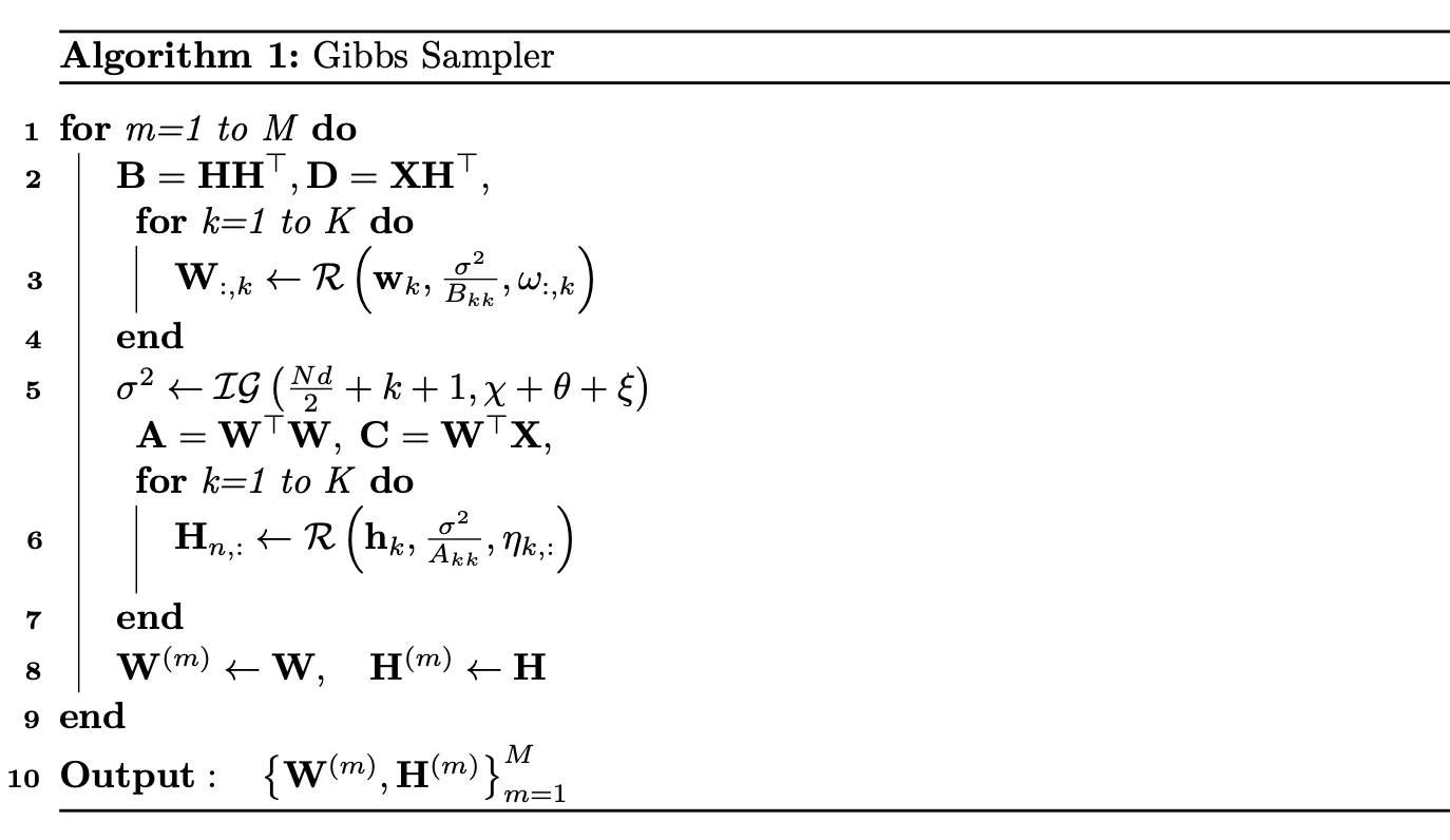
We have derived much of the the theory and equations behind Bayesian NMF in Section 2.2 earlier; however, when implementing this algorithm, there are some key realizations to mention. First, recognize that the elements in each column of \(\mathbf{W}\) and row of \(\mathbf{H}\) are assumed to be conditionally independent, so when implementing the algorithm, we can simply sample an entire column of \(\mathbf{W}\) and row of \(\mathbf{H}\) simultaneously. Further, we leverage matrix computation to avoid inefficient summations, but also, to avoid directly computing large matrices we can strategically define the following,

where the notation \(\mathbf{W}_{:,\setminus k}\) denotes the submatrix of \(\mathbf{W}\) which consists of all columns except the \(k\)-th column. Thus, the most intense computation is comprised of computing the matrix products \(\mathbf{D}\) and \(\mathbf{C}\), which can be pre-computed at each iteration. With these definitions, we can implement an efficient NMF Gibbs sampler as follows,

Examples

We can test the utility of a Gibbs sampler, in the Bayesian NMF framework described earlier, in discerning the factorizing matrices from an observed data matrix. Before testing this method on real data, we can test it on simulated data. There are scarce resources for Bayesian NMF in R, but an implementation of Bayesian NMF detailed in [7] is available in Python at the following GitHub repository. We use this implementation in our simulation study below.

Simulation Study

The BNMF repository includes scripts to generate toy datasets for testing the Bayesian NMF method. We can first use the generate_dataset function to generate a toy dataset; we choose \(N=100, \;d=80, \;K=10\), namely \(\mathbf{X} \in\mathbb{R}^{100\times80}\), with and \(K=10\) latent factors. We can also define priors for both \(\mathbf{W} \in\mathbb{R}^{100\times10}\) and \(\mathbf{H} \in\mathbb{R}^{10\times80}\) to be uniform over all entries. Regarding the noise matrix matrix \(\mathbf{E} \in\mathbb{R}^{100\times80}\), we simply add Gaussian noise with variance true_sigma = 2.5 to each element of \(\mathbf{X}\). Note that as is usually more convenient in the Bayesian framework, we define the precision \(\tau = \sigma^{-2}\), namely the inverse of the variance. We implement this simulation below and show the distribution of the noise added to the observed data matrix. Note that we also take the first 500 iterations as burn-in before calculating the expected model parameters.

import numpy as np
import pandas as pd
import matplotlib.pyplot as plt
import sys
import os
import seaborn as sns
from BNMTF.code.models.nmf_np import NMF
from BNMTF.code.models.bnmf_gibbs_optimised import bnmf_gibbs_optimised
from BNMTF.data_toy.bnmf.generate_bnmf import generate_dataset

project_location = "./"
sys.path.append(project_location) 

# Model parameters
iterations = 2000
burn_in = 500
thinning = 2

# Defining priors
omega, eta = 1., 1.
lambdaW = np.ones((N,K))/10
lambdaH = np.ones((d,K))/10
priors = {'alpha': omega, 'beta':eta, 'lambdaU':lambdaW, 'lambdaV':lambdaH }
mask = np.ones((N,d))

# Simulation parameters
N, d, K = 100, 80, 10    # dimensions
true_sigma = 2.5         # variance
true_tau = 1/true_sigma  # precision
init_WH = 'random'       # random initialization

# Simulate data
W, Ht, true_tau, true_X, X = generate_dataset(N,d,K,lambdaW,lambdaH,true_tau)
H = Ht.T

# Showing noise
plt.hist((true_X - X).flatten(), bins=30)
plt.title("Simulated variance = " + str(round(np.var(true_X - X),4)) + 
  " (true variance = " + str(true_sigma) + ")")
plt.show()

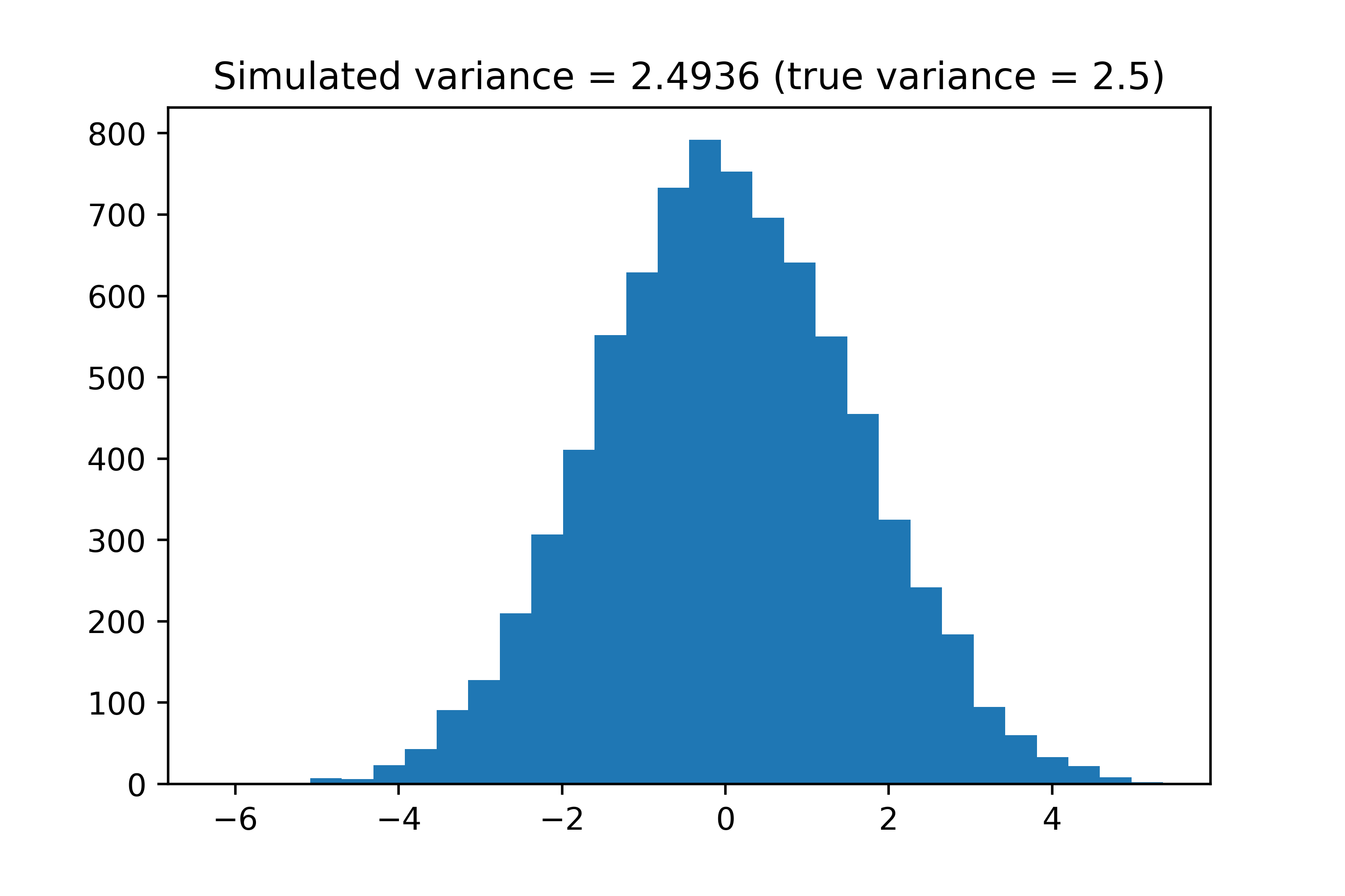
We can confirm that the simulated variance is roughly equal to the true variance defined in this simulation. We can now run the Bayesian NMF method.

# Run the Gibbs sampler
BNMF = bnmf_gibbs_optimised(R=X, M=mask, K=K, priors=priors)
BNMF.initialise(init_WH)
BNMF.run(iterations)

## Iteration 1. MSE: 134294.99267. R^2: 0.47024. Rp: 0.757714. 
## ....
## Iteration 2000. MSE: 2.5096789. R^2: 0.99999. Rp: 0.999995.

# Extracting estimates
burn_in = 500
(exp_W, exp_Ht, exp_tau) = BNMF.approx_expectation(burn_in,thinning)
exp_H = exp_Ht.T
print "True sigma: " + str(true_sigma) + ", Estimated sigma: " + str(1/exp_tau)

## True sigma: 2.5, Estimated sigma: 2.500152611361593

We can further consider the convergence of our parameter values, specifically \(\sigma^2\) and \(\tau\). We consider the traceplots of their value at each iteration of the Gibbs sampler below (excluding the first 100 iterations).

taus = BNMF.all_tau[100:]
sigmas = 1/taus

# Plot tau and sigma against iterations to see that it converges
f, axarr = plt.subplots(3, sharex=True, figsize=(6,8))
x = range(1,len(taus)+1)
axarr[0].set_title('Convergence of values')
axarr[0].plot(x, sigmas)
axarr[0].set_ylabel("Variance, sigma")
axarr[0].axhline(y=true_sigma, color='gray', linestyle='--', label='True sigma')
axarr[0].legend()

axarr[1].plot(x, taus)
axarr[1].set_ylabel("Precision, tau")
axarr[1].axhline(y=true_tau, color='gray', linestyle='--', label='True tau')
axarr[1].legend()

axarr[2].plot(x, BNMF.all_performances['MSE'][100:])
axarr[2].set_ylabel("MSE")
plt.show()

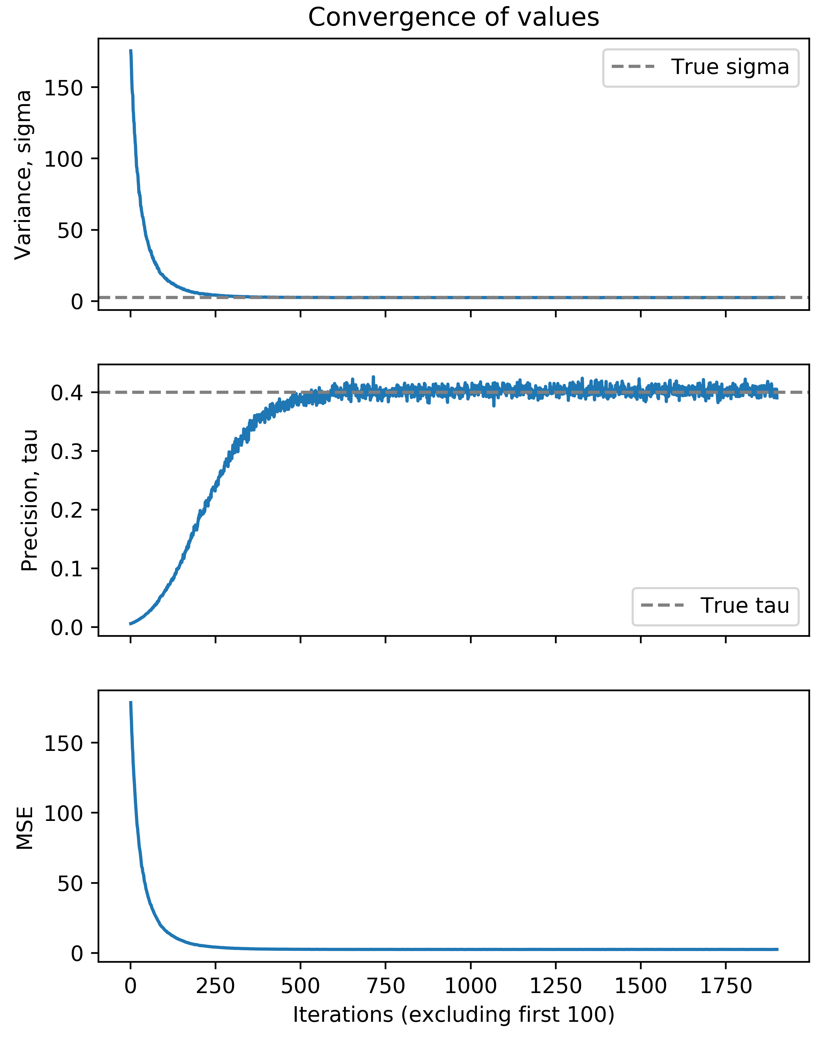
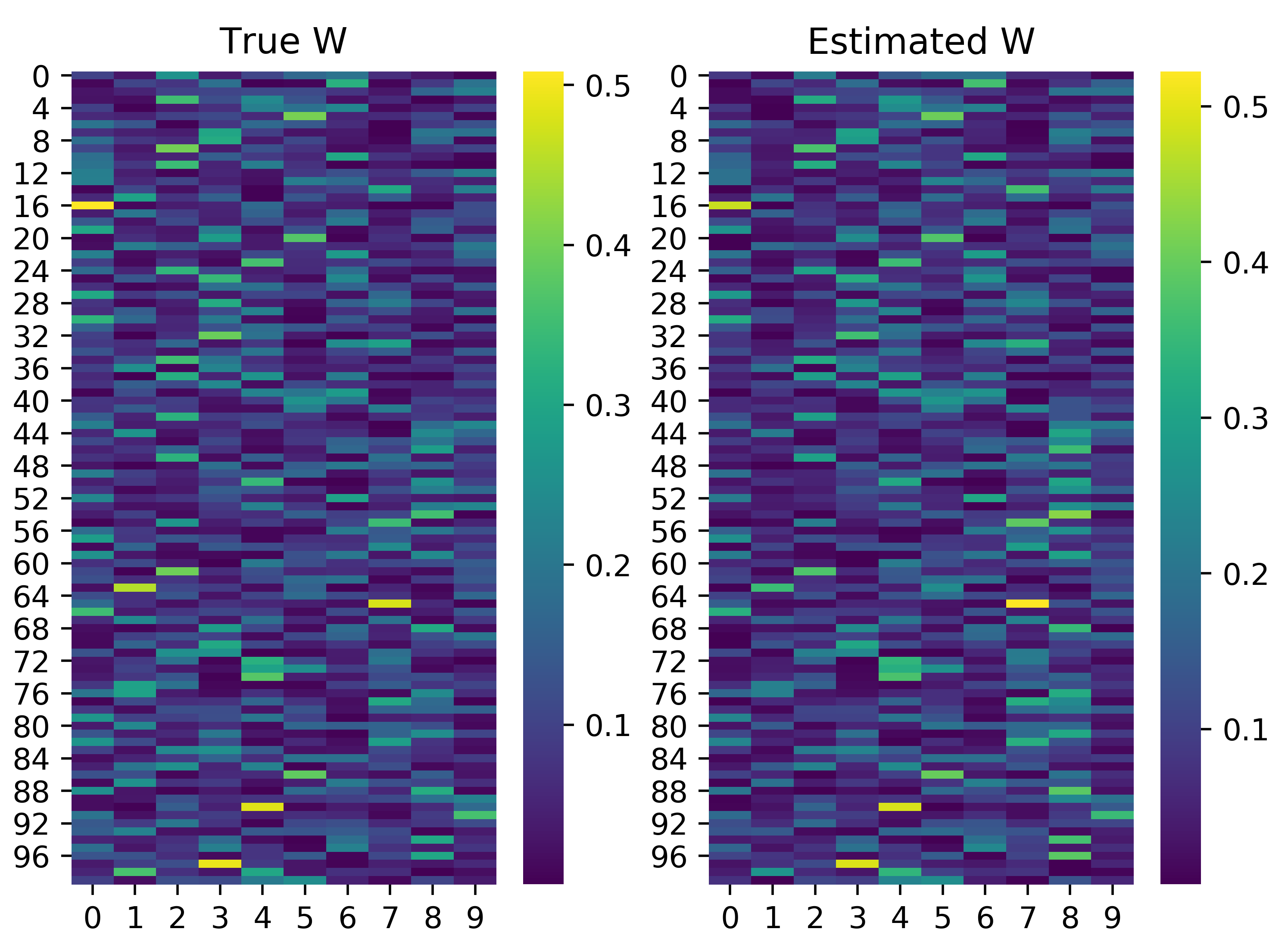
We see that after roughly 500 iterations of the Gibbs sampler, we converge on the true value of \(\tau\) and \(\sigma\). We can also evaluate the other two parameters of the Bayesian NMF model, namely the factorizing matrices \(\mathbf{W}\) and \(\mathbf{H}\). Note that the estimated factors are not necessarily the same order as in the true factorizing matrices, so we must infer the proper order. We can simply match columns in \(\mathbf{W}\) or rows in \(\mathbf{H}\) by considering the minimum summed squared difference across the two matrices. We can implement this idea and visualize the results below. Note that we normalize the columns in \(\mathbf{W}\) and rows in \(\mathbf{H}\) to simply allow for reasonable comparison.

def find_rowOrder_min(mat1, mat2):
    order = []
    for i1 in range(mat1.shape[1]):
        all_comp = np.zeros((mat2.shape[1]))
        for i2 in range(mat2.shape[1]):
            all_comp[i2] = np.square(mat1[:, i1] - mat2[:, i2]).sum()
        order.append(np.argmin(all_comp))
    return(np.array(order))

def find_colOrder_min(mat1, mat2):
    order = []
    for i1 in range(mat1.shape[0]):
        all_comp = np.zeros((mat2.shape[0]))
        for i2 in range(mat2.shape[0]):
            all_comp[i2] = np.square(mat1[i1, :] - mat2[i2, :]).sum()
        order.append(np.argmin(all_comp))
    return(np.array(order))

# normalize rows for comparison
W_norm = W/W.sum(axis=1, keepdims=True)
exp_W_norm = exp_W/exp_W.sum(axis=1, keepdims=True)
exp_W_norm = exp_W_norm[:,find_rowOrder_min(W_norm, exp_W_norm)]

fig, (ax1, ax2) = plt.subplots(1,2)
sns.heatmap(W_norm, cmap = 'viridis', ax=ax1)
ax1.set_title('True W')
sns.heatmap(exp_W_norm, cmap = 'viridis', ax=ax2)
ax2.set_title('Estimated W')
plt.show()

# normalize rows for comparison
H_norm = H/H.sum(axis=0, keepdims=True)
exp_H_norm = exp_H/exp_H.sum(axis=0, keepdims=True)
exp_H_norm = exp_H_norm[find_colOrder_min(H_norm, exp_H_norm),:]

fig, (ax1, ax2) = plt.subplots(1,2, figsize=(12,2))
sns.heatmap(H_norm, cmap = 'viridis', ax=ax1)
ax1.set_title('True H')
sns.heatmap(exp_H_norm, cmap='viridis', ax=ax2)
ax2.set_title('Estimated H')
plt.show()

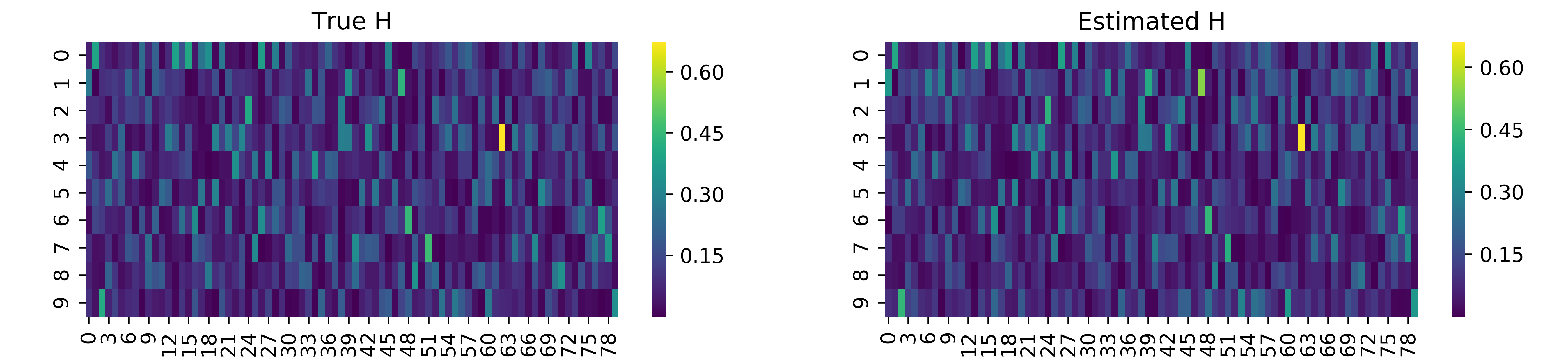
We also see here that the factorizing matrices estimated are actually fairly accurate. “Hotspots”, or cells with high value, in the heatmap above roughly match in the estimated and true factorizing matrices. Thus, we have demonstrated the utility of Bayesian NMF in discerning the factorizing matrices from observed data.

Note that if we did not assume \(K\) was known, we could perform model selection by considering the log-likelihood across several values of \(K\). As \(K\) increases, we expect the log-likelihood to continue increasing, even if marginally, as we give the model more freedom to fit the data; however, this can lead to over-fitting. We can thus penalize the the model’s performance by its complexity. We can consider the Akaike information criterion (AIC) defined as,

where \(\Psi\) is the number of free parameters in our model. In NMF, this is simply the number of elements in \(\mathbf{W}\) and \(\mathbf{H}\), namely \(NK + Kd\). We can run Bayesian NMF for \(K=5,\dots,14\) and plot the log-likelihood and AIC for the expected model parameters after the Gibbs sampler converges.

# calculate AIC
AIC = []
for i,k in enumerate(range(5,15)):
    AIC.append(2*(k*N + k*d) - 2*final_log_likelihood[i])

ax1 = sns.scatterplot(range(5,15), AIC, s=50)
ax2 = ax1.twinx()
sns.scatterplot(range(5,15), final_log_likelihood, s=50, ax=ax2, color='red')
sns.lineplot(range(5,15), AIC, ax=ax1)
sns.lineplot(range(5,15), final_log_likelihood, ax=ax2, color='red')
ax1.set_ylabel("AIC")
ax2.set_ylabel("Log-likelihood")
ax1.set_xlabel("Number of factors, K")
plt.title('Red: AIC, Blue: Log-likelihood')
plt.show() 

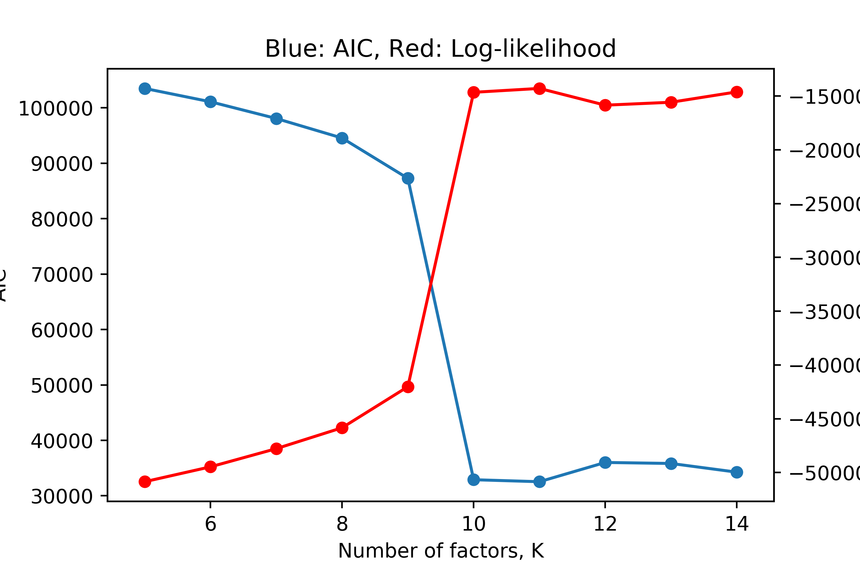
We see that this “brute-force” or greedy model selection does in fact show the correct answer. We see a sharp increase in log-likelihood and decrease in AIC at \(K=10\), followed by a plateau, indicating that \(K=10\) is the optimal number of factors under this model, which is correct.

Olivetti Faces Dataset

We apply Bayesian NMF to the Olivetti faces dataset, which containsa a set of face images taken between April 1992 and April 1994 at AT&T Laboratories Cambridge. The dataset includes 400 different images of 40 distinct subjects. Images of subjects were taken at different times, varying the lighting, facial expressions, and facial details (e.g. glasses or no glasses). We select \(K=10\) here based on prior beliefs; however, model selection should be performed to be more rigorous here.

Due to the non-negativity constraints of NMF, we would expect the features it learns, namely the rows of \(\mathbf{H}\), to be key features of a face, which can be weighted by the values in \(\mathbf{W}\) to reconstruct the original faces in the dataset. This is especially in contrast to a method like PCA, which allows for subtraction across features; the features that we expect PCA to learn may not necessarily be specific features of the face since feature subtractions can be used to reconstruct the face images. We run both Bayesian NMF and PCA below

# Load the faces datasets
data = sklearn.datasets.fetch_olivetti_faces()
data.data.shape

# PCA (using SVD)
Xc = X/np.mean(X, axis=0)
U, s, Vt = np.linalg.svd(Xc)
Vt.shape

plt.plasma()
plt.figure(figsize=(2,5))
rows, cols = 2, 5
fig, axes = plt.subplots(nrows=rows, ncols=cols, figsize=(15,6.2))
cnt = 0
for i in range(rows):
    for j in range(cols):        
        axes[i,j].imshow(Vt[cnt,:].reshape((64,64)))
        axes[i,j].set_title('Feature '+str(cnt))
        cnt += 1

# Bayesian NMF
X = data.data
N, d = X.shape
K = 10
iterations = 200
burn_in = 150

# Defining priors
omega, eta = 1., 1.
lambdaW = np.ones((N,K))/10
lambdaH = np.ones((d,K))/10
priors = {'alpha': omega, 'beta':eta, 'lambdaU':lambdaW, 'lambdaV':lambdaH }
mask = np.ones((N,d))

# Run the Gibbs sampler
BNMF = bnmf_gibbs_optimised(R=X, M=mask, K=K, priors=priors)
BNMF.initialise(init_WH)
BNMF.run(iterations)
(exp_W, exp_Ht, exp_tau) = BNMF.approx_expectation(burn_in,thinning)
exp_H = exp_Ht.T

plt.figure(figsize=(2,5))
rows, cols = 2, 5
fig, axes = plt.subplots(nrows=rows, ncols=cols, figsize=(15,6.2))
cnt = 0
for i in range(rows):
    for j in range(cols):        
        axes[i, j].imshow(exp_H[cnt].reshape((64,64)))
        axes[i,j].set_title('Feature '+str(cnt))
        cnt += 1

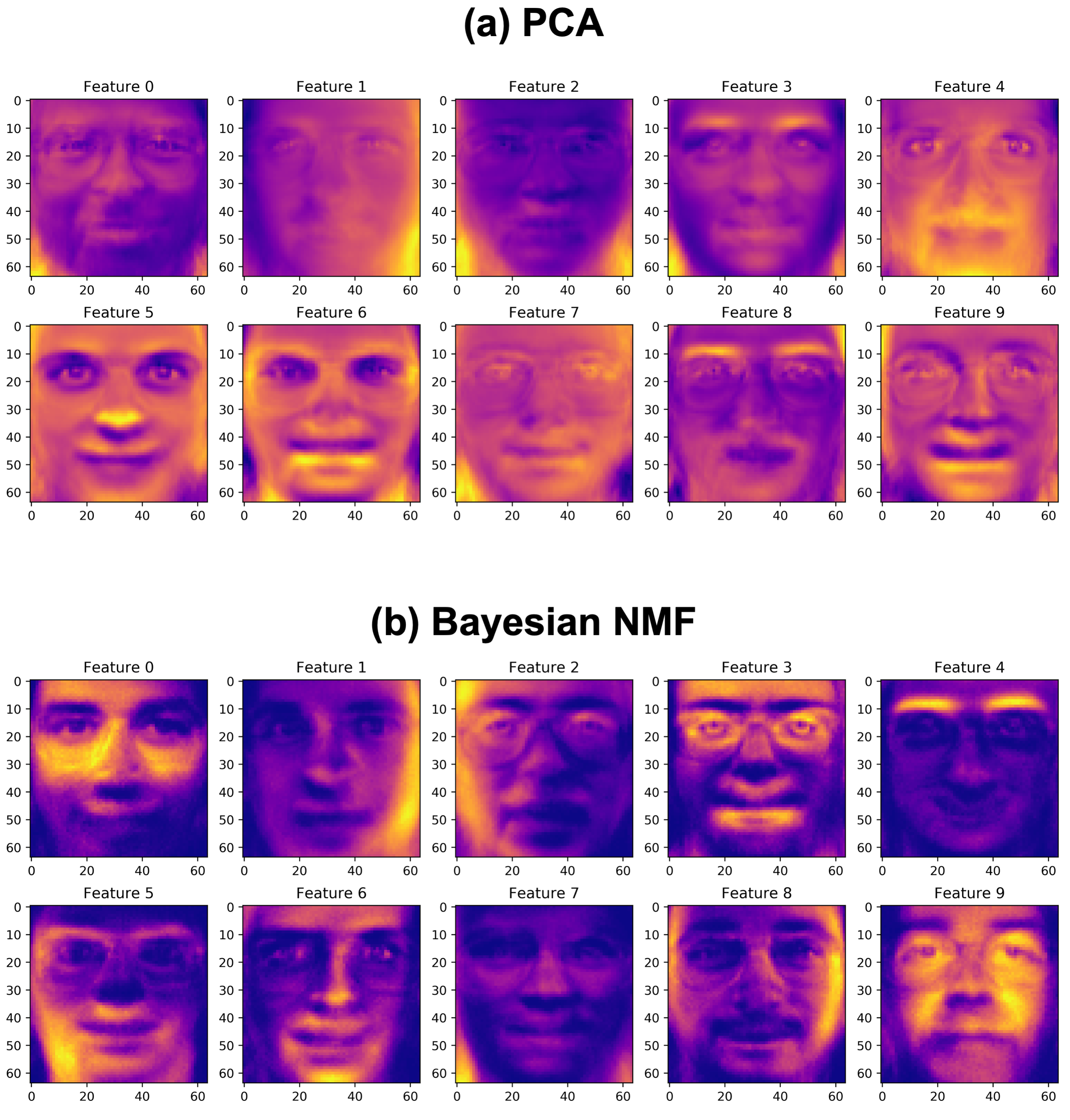
We see that as we expected, the Bayesian NMF method picks up specific features of a face (“puzzle-pieces”) which can be added to reconstruct the original faces in the dataset. Perhaps the best example of this is Feature 4 above, which very clearly represents the eyebrows in the data. Likewise, Feature 6 seems to have picked up the chin, Feature 1 picks up glasses, Feature 8 picks up the outside of the face, and so on. Comparing this to PCA, we see that the features learned by PCA are not nearly as intuitive. The features may add and subtract to reconstruct the faces in the original dataset, but the features themselves do not represent building blocks of the face, similar to in Bayesian NMF. This notion of intuitive features is a very clear advantage of Bayesian NMF (and NMF in general), which results from the non-negativity constraints applied.

MNIST Dataset

The MNIST database (Modified National Institute of Standards and Technology) is an extensive database of handwritten digits that is commonly used in the field of unsupervised learning [8]. Here, we implement Bayesian NMF on a small subset of 10,000 images from this MNIST database available on Kaggle. Similar to before, here, we expect the features learned to be key features of a digit, such as key curves or contours associated with a specific image.

We can also consider more closely the estimated \(\mathbf{W}\) matrix here, which can be interpreted as a matrix of weights for the features defined by the \(\mathbf{H}\) matrix. Since we expect each number class in the dataset to be defined by some addition of the features that NMF learns, then we can assign each data point to the factor or factors, which it weights highly. Essentially, we can “assign” a given point, namely a row in the matrix \(\mathbf{W}\), to the cluster which corresponds to the highest weight in that row. Doing this has the effect of clustering the data, and we would expect each cluster to roughly correspond to 1-2 images. Below, we learn MNIST features using Bayesian NMF, and cluster the data using the method just described. Note that this method draws inspiration from the biological applications of NMF, where genes might be assigned to certain gene batteries for example.

d = pd.read_csv('./MNIST/mnist_test.csv')
labels = d.iloc[:,0].to_numpy()
data = d.iloc[:,1:].to_numpy()

# Bayesian NMF
X = data
N, d = X.shape
K = 10
iterations = 200
burn_in = 150

# Defining priors
omega, eta = 1., 1.
lambdaW = np.ones((N,K))/10
lambdaH = np.ones((d,K))/10
priors = {'alpha': omega, 'beta':eta, 'lambdaU':lambdaW, 'lambdaV':lambdaH }
mask = np.ones((N,d))

# Run the Gibbs sampler
BNMF = bnmf_gibbs_optimised(R=X, M=mask, K=K, priors=priors)
BNMF.initialise(init_WH)
BNMF.run(iterations)
(exp_W, exp_Ht, exp_tau) = BNMF.approx_expectation(burn_in,thinning)
exp_H = exp_Ht.T

# Extract featuresplt.figure(figsize=(2,5))
plt.plasma()
rows, cols = 2, 5
fig, axes = plt.subplots(nrows=rows, ncols=cols, figsize=(18,7))
cnt = 0
for i in range(rows):
    for j in range(cols):        
        axes[i, j].imshow(exp_H[cnt].reshape((28,28)))
        axes[i,j].set_title('Feature '+str(cnt))
        cnt += 1

# "Clustering"
exp_W_norm = exp_W / np.sum(exp_W, axis = 1, keepdims=True)
assigns = np.argmax(exp_W, axis=1)
mean_clust = np.zeros((K, d))
tt = []
for i in range(K):
    idx = np.where(assigns == i)
    mean_clust[i] = np.mean(X[idx,:], axis=1)
    sz = len(idx[0])
    val, cnts = np.unique(labels[idx], return_counts=True)
    lab, contrib = val[cnts > sz/4.], cnts[cnts > sz/4.]
    if(len(contrib) == 0):
        lab, contrib = val[cnts == max(cnts)], cnts[cnts == max(cnts)]
    str_t = ", ".join([str(i)+": "+str(round(100.*j/float(sz),2))+"%" for i,j in zip(lab, contrib)])
    tt.append(str_t+" (size "+str(sz)+")")

plt.figure(figsize=(2,5))
rows, cols = 2, 5
fig, axes = plt.subplots(nrows=rows, ncols=cols, figsize=(18,7))
cnt = 0
for i in range(rows):
    for j in range(cols):        
        axes[i,j].imshow(mean_clust[cnt].reshape((28,28)))
        axes[i,j].set_title(tt[cnt])
        cnt += 1

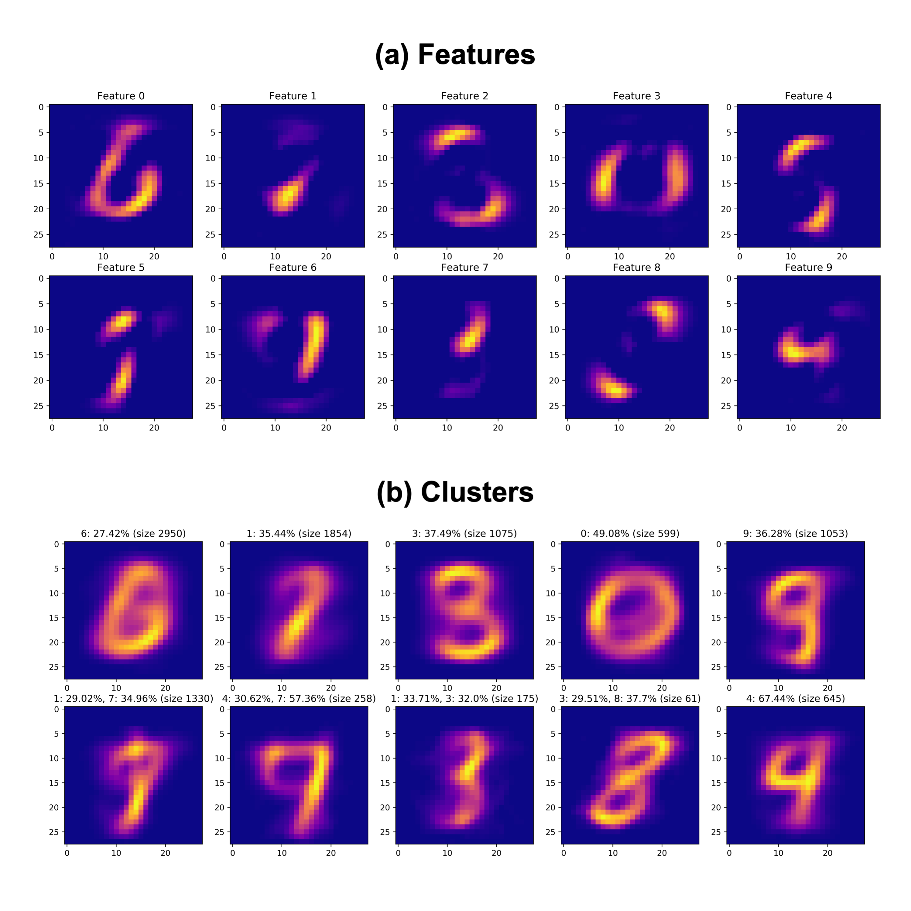
We see that the features and clusters above do in fact roughly correspond to the different images in the MNIST dataset. Above each cluster, we include the high contributors to each of the clusters. The features themselves seem to be key elements of a digit image, such as the curve of a “6” digit in Feature 0. Further, aligning the features to clusters above, we can see that each feature roughly corresponds to a cluster, specifically indicated by the brighter regions in each feature. These results again demonstrate the utility of Bayesian NMF in discerning a small subset of important representative features of a dataset.

Discussion

Strengths

Here, we discuss Bayesian NMF, which has a variety of advantages over the original NMF algorithm introduced by Lee and Seung [1]. In particular, prior knowledge can be incorporated into the factorization process, which may improve the quality of the resulting factorization by incorporating domain-specific knowledge and reducing overfitting [4]. Incorporating prior beliefs in the factorization process will also dramatically reduce the convergence time for the Gibbs sampler; this is a great advantage over regular NMF which converge relatively slowly by coordinate descent. The incorporation of prior beliefs can also be considered as regularization during the factorization process, thereby making Bayesian NMF more robust to noise.

A particularly useful feature of Bayesian NMF is its ability to provide uncertainty estimates for the factors. Uncertainty estimation and out-of-distribution robustness are critical issues to address in the context of machine learning. For example, in medical applications, an over-confident misprediction, namely with an inaccurate uncertainty estimate, may result in a misdiagnosis that is not subsequently considered by a physician as a result. This can clearly have disastrous consequences [9]. Thus, by providing uncertainty estimates for the factors, Bayesian NMF offers more interpretable resulting factors.

The Gibbs sampling procedure introduced can also directly be used to estimate the marginal likelihood, which is useful for model order selection. Further, the ICM algorithm discussed briefly for computing the MAP estimate has been shown to rival even existing state-of-the-art NMF algorithms [4].

Ultimately, Bayesian NMF and the original NMF algorithm offer a variety of advantages in allowing for decomposition of a data matrix into a product of two lower-rank matrices. In particular, this can be useful for data compression, feature extraction, and dimensionality reduction. Bayesian NMF can provide a compact and more interpretable representation of the data, which can used downstream for techniques such as clustering (demonstrated here), classification, and visualization. In addition, the low-rank structure of the resulting factorizing matrices provides valuable insight into the underlying structure of the data, thereby facilitating the discovery of latent patterns and trends in the data.

Weaknesses

NMF is a widely-used method for extracting meaningful and more interpretable feature decompositions from non-negative data sets, and this non-negativity constraint is both natural and relevant to a wide variety of contexts as discussed earlier. However, its lack of flexibility for negative data values may limit its performance in some applications.

Specifically, Bayesian NMF is also fairly sensitivity to the priors and initialization selected, and as a result, it may converge to suboptimal solutions, making it difficult to obtain consistent results with NMF. The lack of a closed-form analytical solution is a clear weakness which demands iterative methods in the case of NMF or MCMC methods in the case of Bayesian NMF here. In particular, this makes Bayesian NMF prone to local optima solutions; selecting appropriate priors or starting from several random initializations and subsequently considering the log-likelihood are useful strategies to avoid non-global optima solutions.

While the methods introduced here, in particular the Gibbs sampler and ICM, are great techniques for achieving faster convergence (sometimes even faster than the original NMF algorithm), computational complexity is surely a weakness in the Bayesian inference framework. This can make it particularly challenging to apply Bayesian NMF to large data sets.

References

[1] Lee, D., & Seung, H. S. (2000). Algorithms for non-negative matrix factorization. Advances in Neural Information Processing Systems, 13.

[2] Gaussier, E., & Goutte, C. (2005). Relation between PLSA and NMF and implications. Proceedings of the 28th Annual International ACM SIGIR Conference on Research and Development in Information Retrieval, 601–602.

[3] Sherman, T. D., Gao, T., & Fertig, E. J. (2020). CoGAPS 3: Bayesian non-negative matrix factorization for single-cell analysis with asynchronous updates and sparse data structures. BMC Bioinformatics, 21(1), 1–6.

[4] Schmidt, M. N., Winther, O., & Hansen, L. K. (2009). Bayesian non-negative matrix factorization. International Conference on Independent Component Analysis and Signal Separation, 540–547.

[5] Chib, S. (1995). Marginal likelihood from the gibbs output. Journal of the American Statistical Associa- tion, 90(432), 1313–1321.

[6] Besag, J. (1986). On the statistical analysis of dirty pictures. Journal of the Royal Statistical Society: Series B (Methodological), 48(3), 259–279.

[7] Brouwer, T., Frellsen, J., & Lio, P. (2016). Fast bayesian non-negative matrix factorisation and tri- factorisation. arXiv Preprint arXiv:1610.08127.

[8] LeCun, Y. (1998). The MNIST database of handwritten digits. Http://Yann. Lecun. Com/Exdb/Mnist/.

[9] Dusenberry, M. W., Tran, D., Choi, E., Kemp, J., Nixon, J., Jerfel, G., Heller, K., & Dai, A. M. (2020). Analyzing the role of model uncertainty for electronic health records. Proceedings of the ACM Conference on Health, Inference, and Learning, 204–213.