Setting

In this project, we evaluate the ranking of NFL quaterbacks by several expert rankers. We have the ranking lists of the NFL starting quarterbacks from 13 experts in week 12 of season 2014 as well as some summary statistics of the players. While most experts give similar ranking lists, some rankings might be missing, and differences do exist. Further, it is important to understand how the rankings may be dependent of the available summary statistics. Here, we attempt to arrive at an aggregated ranking list of all players taking into account the available covariate information and potential heterogeneity among expert rankings.

We consider the following latent regression model. For a given set of \(M\) ranking lists, \(\boldsymbol\tau = \{\tau_1, \dots, \tau_M\}\), with respect to \(N\) entities (namely, NFL quarterbacks), \(\mathcal{U} = \{1,2, \dots, N\}\). We assume that behind each ranking list, there exists some latent random vector \(\mathbf Z_j = (Z_{1j}, \dots, Z_{Nj})^\top\), where \(Z_{ij}\) represents ranker \(j\)’s evaluation score of the \(i\)th entity, and \(Z_{i_1j} > Z_{i_2j} \iff i_1 \succ i_2\), namely if and only if ranker \(j\) ranks player \(i_1\) ahead of player \(i_2\). So, we have \(\tau_j = \text{rank}(\mathbf Z_j)\), where we again note that \(\tau_j(i_1) < \tau_j(i_2) \iff i_1 \succ i_2\). We also define \(\mathbf Z_i = (Z_{i1}, \dots, Z_{iM})^\top\) as the score evaluations received by player \(i\) across the \(M\) expert rankers. We can thus construct a matrix of all the \(Z_{ij}\). Let this \(N\times M\) matrix be \(\mathbb{Z}\), where the \(i\)th row is \(\mathbf Z_i\) and the \(j\)th column is \(\mathbf Z_j\).

Also let \(\mathbf x_i = (x_{i1}, \dots, x_{ip})^\top\) denote the covariates available for the \(i\)th player, and let \(\boldsymbol\beta = (\beta_1, \dots, \beta_p)^\top\) be the vector of coefficients. Similar to before, we define the matrix \(\mathbf X\), where the rows are the \(\mathbf x_i^\top\). Our full data model then takes the following form:

for \(i = 1, \dots, N\) and \(j = 1, \dots, M\). We view the \(\alpha_i\) as random effects of each entity.

With the model specified, we can begin by loading and organizing the data below.

t1 = read.table("Table1_RankingList.csv", header=TRUE, row.names=1, sep=",")
t2 = read.table("Table2_SummaryStatistics.csv", header=TRUE, row.names=1, sep=",")

N = nrow(t1)
M = ncol(t1)
p = ncol(t2)
X = scale(as.matrix(t2))

Part 1

Is it reasonable to assume that \(\text{Var}(\epsilon_{ij}) = 1\) in the model? Can you just assume an unknown variance \(\sigma^2\) for it and try to infer it from the data? Why or why not?

Here, we are interested in inferring an aggregated ranking list of all players taking into account the available covariate information as well as the heterogeneity among expert rankings. Since the rank is invariant to scaling, the absolute value of the error variance in the model does not directly affect the inference of the rank \(\tau_j\).

Explicitly, we have \(\mathbf Z_j = \boldsymbol\alpha + \mathbf X \boldsymbol\beta + \boldsymbol\epsilon_j\), meaning that \(\text{Cov}(\mathbf Z_j) = \sigma^2_a\mathbb I_N + \sigma^2_b\mathbf X^\top \mathbf X + \mathbb I_N\). The random effects \(\alpha_i\) here account for the variability across players, and the \(\sigma^2_b\) accounts for the variability on the covariates coefficients (assuming they have variance \(\sigma^2_b\) as in Part 2). Thus, we see that the primary purpose of the error term \(\epsilon_{ij}\) here is to capture the unexplained variability between the rankings of the same player. Based on the data from Table 1, it is not unreasonable to assume that this variability is small, and assuming that \(\text{Var}(\epsilon_{ij}) = 1\) simplifies the model without affecting the inference of the rank, while still capturing any additional variance needed between the observations. Further, note that any additional variance needed to explain the data can simply be accounted for by the \(\sigma^2_a\) from the random effect. So, it seems reasonable to assume a constant error variance and focus on inferring the rank and other model parameters.

Further, assuming an unknown variance \(\sigma^2\) for \(\text{Var}(\epsilon_{ij})\) and trying to infer it from the data will not necessarily work well since we never actually assume the \(Z_{ij}\). These are in fact latent variables. Given that we only see the rank of the \(Z_{ij}\), and rank is invariant of scaling, assuming \(\text{Var}(\epsilon_{ij}) = 1\) is actually a very reasonable and viable strategy.

Part 2

We now Assume that \(\sigma^2_a \sim \text{Inv-}\chi^2(\nu_a, s^2_a)\), with \(\nu_a\) and \(s^2_a\) being values fixed or tuned by the user. We also assume that \(\beta_j \sim\mathcal{N}(0, \sigma^2_b)\), again with \(\sigma^2_b\) being a tuning hyperparameter input by the user. We want to write down the joint distribution of all the unknown parameters, the latent variables \(\mathbf Z_j\), and the observed ranking lists \(\tau_j\) in the model.

We can start by drawing the full data model in graphical representation to clearly see any conditional independence structures that may be useful in the data. We have,

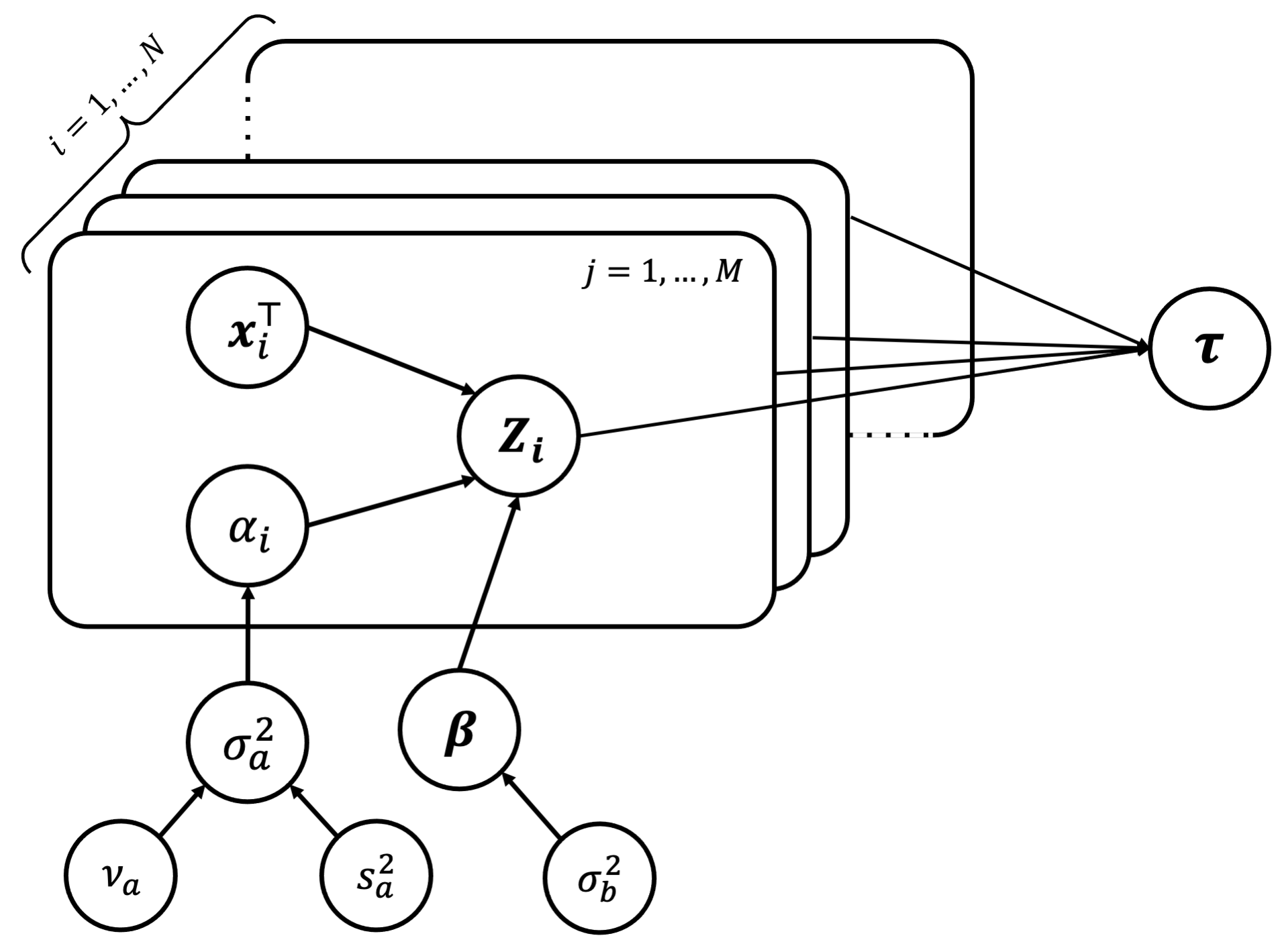
Using this, we can write down the joint distribution of all the unknown parameters. We have,

In the expression below, we have the distribution of each term. First, note that for \(p(\boldsymbol\tau\\|\mathbb Z)\), given \(\mathbb Z\), \(\tau_j\) is simply the rank (deterministic) function. We can thus represent this probability distribution as a function of indicators,

For the second factor \(p(\mathbb{Z}\\| \boldsymbol\beta,\boldsymbol\alpha, \mathbf X)\), first note that the \(\mathbf Z_i\) are independent across players since the \(\alpha_i\) are drawn iid. So we have,

Note that combined with the first factor, we note that we have a Truncated Normal distribution for each \(Z_{ij}\), where each \(Z_{ij}\) is Normally distributed with mean \(\alpha_i + \mathbf x_i^\top\boldsymbol\beta\) and variance 1, but with upper and lower bounds given by the \(Z_{kj}\) with one lower and one higher rank, respectively.

For the remaining factors in the joint distribution, we have \(p(\boldsymbol\alpha) = \prod_{i=1}^N \mathcal{N}(\alpha_i; 0, \sigma^2_a)\), as well as \(p(\sigma^2_a\\|\nu_a, s^2_a) = \text{Inv-}\chi^2(\nu_a, s^2_a)\) and \(p(\boldsymbol\beta\\|\sigma^2_b) = \prod_{k=1}^p\mathcal{N}(\beta_k; 0, \sigma^2_b)\). So, our full data joint can be written together as,

Part 3

Explain in detail how the joint distribution obtained above takes care of missing ranking information.

In the joint distribution above, we importantly include the latent variables \(\mathbf Z_j\), which incorporate the evaluation score for ranker \(j\) across all the \(N\) entities/players. In the joint above, we have the condition that \(\tau_j(i_1)<\tau_j(i_2)\iff i_1\succ i_2\) by raising the two indicator functions to each other. If the ranking information for a given player is not available by one of the rankers, ranking condition on \(\tau\) may still hold (thereby not “zeroing out” the joint), and we can then estimating the latent \(Z_{ij}\) for the missing player, thereby allowing us to add or impute their rank for ranker \(j\). For this missing player, as discussed in part 2, \(Z_{ij}\) will in fact be a Truncated Normal whose upper bound is the player ranked directly above and whose lower bound in the player ranked directly under. Note that this \(Z_{ij}\) can be estimated for a missing \(ij\)th ranking since we assume that heterogeneity among rankers for the \(i\)th player, namely \(\mathbf Z_i\), is simply a result of unit variance on \(\boldsymbol\epsilon_i\).

Part 4

Under the same prior assumptions as in Part 2, we can consider a data augmentation-based strategy and derive all conditional distributions necessary for implementing a Gibbs sampling algorithm to sample from the joint posterior distribution of all the unknown parameters and the latent variables \(\mathbf Z_j\). We will take advantage of the avrious conditional independence properties, illustrated by the graphical model (d-separation/blocking rules). First consider the full conditional distribution for \(\sigma_a^2\). We have,

We can use the well-known Normal-Inv-\(\chi^2\) conjugacy (see Section 2.6 in BDA) to see that

Now, consider the full conditional distribution for \(\boldsymbol\alpha\). We have,

We can simplify this conditional by taking advantage of the fact that the random effects are drawn iid from the same distribution, thereby allowing us to update each of the \(N\) components of \(\boldsymbol\alpha\) independently. Namely, we can evaluate \(p(\mathbf{Z}_i \\| \boldsymbol\beta, \mathbf X, \alpha_i)\) by considering this as \(M\) draws from the \(\mathcal{N}(\alpha_i + \mathbf x_i^\top \boldsymbol\beta,1)\) distribution, corresponding to the \(M\) rankings:

However, we can also think of the \(\mathbb{Z}\) as \(M\) draws from an \(N\)-dimensional Multivariate Normal distribution with mean vector \(\boldsymbol\alpha + \mathbf X\boldsymbol\beta\) and the following covariance matrix,

Define \(\boldsymbol\Sigma := \text{Cov}(\mathbf Z_j) = \sigma^2_b\mathbf X^\top \mathbf X + (\sigma^2_a + 1)\mathbf I_N\). Likewise, since the \(\alpha_i\) are iid, we have, \(\boldsymbol\alpha\\|\sigma^2_a \sim \mathcal{N}(\mathbf 0, \sigma^2_a\mathbf I_N)\). By the multivariate Normal-Normal conjugacy result, we have,

where by completing the square, we have,

Now, consider the full conditional distribution for \(\boldsymbol\beta\). We have,

We cannot necessarily directly apply the Normal-Normal conjugacy result here since \(\boldsymbol\beta\) is \(p\)-dimensional, while the \(\mathbf{Z}_i\) are \(M\)-dimensional vectors. In other words, each player does not only update one component independently as with \(\boldsymbol\alpha\); instead, each player or score evaluation \(Z_{ij}\) updates \(\boldsymbol\beta\) slightly. To derive this conditional distribution, we can again think of the \(\mathbb{Z}\) as \(M\) draws from an \(N\)-dimensional Multivariate Normal distribution with mean vector \(\boldsymbol\alpha + \mathbf X\boldsymbol\beta\) and covariance matrix \(\boldsymbol\Sigma\). This way, we can iteratively update the conditional distribution of \(\boldsymbol\beta\) based on each ranking; each updated posterior for \(\boldsymbol\beta\) is treated as the prior when updating based on the next ranking. Consider for generality \(\boldsymbol\beta \sim \mathcal{N}(\boldsymbol\beta_0, \Lambda_0)\). We can derive the posterior by completing the square in multiple dimensions. Again, let all \(d_i\) represent constants,

where

By recursively updating \(\boldsymbol\beta\) using on the \(M\) rankings, we can arrive at the full conditional distribution for \(\boldsymbol\beta\) based on \(\mathbf Z_1, \dots, \mathbf Z_j\). Note that we might consider updating our \(\boldsymbol\beta\) all at once in the conditional by using the row means of \((\mathbb Z - \boldsymbol\alpha\mathbf1^\top)\) in place of \((\mathbf Z_j - \boldsymbol\alpha)\) in the posterior covariance expression above (since means are sufficient in Normal likelihoods).

Now, consider the full conditional distribution for \(\mathbb Z\). We have,

where the notation \(Z_{kj}(\tau_j(i+1))\) refers to the latent score assigned to player \(k\) who is ranked at \(i+1\) by ranker \(j\). So, we have Truncated Normal distributions for the \(Z_{ij}\) conditional distributions.

Finally, recognize that the full conditional distribution of \(\boldsymbol\tau\) is simply \(p(\boldsymbol\tau\\|\mathbb Z)\) as illustrated by the blocking in the graphical model. We found this distribution in Part 2, but essentially we have by construction \(\tau_j = \text{rank}(\mathbf Z_j)\), which is how we will update the \(\boldsymbol\tau\) matrix in our Gibbs sampler implementation in the next Part. Essentially, we will iteratively draw samples from each conditional distribution to approximate draws from the joint posterior distribution.

Part 5

Using the conditional distributions from Part 4, we can now implement a Gibbs sampler we derived above to sample from the joint posterior distribution. We first write functions to draw from each conditional distribution derived in Part 4.

# Compute conditional distribution of Z: Truncated Normal
compCond_Z = function(tau, Z, alpha, beta, X){
    for (j in 1:M) {
    for (i in 1:N) {
        r_ij = tau[i, j]
        
        # find lower and upper bounds for TN
        L = ifelse(r_ij==1, yes = -Inf, no = sort(Z[,j])[r_ij-1])
        U = ifelse(r_ij==N, yes = Inf, no = sort(Z[,j])[r_ij+1])
        
        Z[i,j] = truncnorm::rtruncnorm(1, mean = alpha[i] + X[i,] %*% beta, 
                                        sd = 1, a = L, b = U)
    }
    }
    return(Z)
}

# Compute conditional distribution of tau: rank
compCond_tau = function(Z) return(apply(Z, 2, rank))

# Compute conditional distribution of beta: Multivariate Normal (recursive strategy)
compCond_beta = function(Z, alpha, X, sig2_b, sig2_a){
    M = ncol(Z); N = nrow(Z); p = ncol(X)
    Sigma_inv = solve(sig2_b * X %*% t(X) + (sig2_a+1) * diag(N))
    Lambda0_inv = diag(p)/sig2_b
    beta0 = matrix(0, nrow = ncol(X), ncol = 1)
    
    # update beta components iteratively based on the Z_j
    Lambda_inv = Lambda0_inv; beta = beta0
    for(j in 1:M){
    Lambda_inv = t(X) %*% Sigma_inv %*% X + Lambda_inv
    Lambda = solve(Lambda_inv)
    beta = Lambda %*% (t(X) %*% Sigma_inv %*% (Z[,j] - alpha) + Lambda_inv %*% beta)
    }
    #Z_cntrd = rowSums(apply(Z, 2, function(x) x - c(alpha)))
    #Lambda = solve(t(X) %*% Sigma_inv %*% X + Lambda0_inv)
    #beta = Lambda %*% (t(X) %*% Sigma_inv %*% Z_cntrd + Lambda0_inv %*% beta0)
    
    draw = mvtnorm::rmvnorm(n=1, mean = beta, sigma = Lambda)
    return(t(draw))
}

# Compute conditional distribution of alpha: Normal (component by component)
compCond_alpha = function(Z, beta, X, sig2_a, sig2_b){
    M = ncol(Z); N = nrow(Z)
    Sigma_inv = solve(sig2_b * X %*% t(X) + (sig2_a + 1) * diag(N))
    barZ = as.numeric(apply(Z, 1, mean))
    
    SigmaN_inv = M * Sigma_inv + diag(N)/sig2_a
    SigmaN = solve(SigmaN_inv)
    alpha = SigmaN %*% (M * Sigma_inv %*% (barZ - X %*% beta) )
    
    # for(i in 1:N){
    #   mean_i = (sum(Z[i,]) - M * X[i,] %*% beta)/(1/sig2_a + M)
    #   var_i = 1/(1/sig2_a + M)
    #   alpha[i] = rnorm(1, mean_i, sqrt(var_i))
    # }
    draw = mvtnorm::rmvnorm(n=1, mean = alpha, sigma = SigmaN)
    return(t(draw))
}

# Compute conditional distribution of sig2_a: Inv-chi^2
compCond_sig2a = function(alpha, nu_a, s2_a){
    N = length(alpha)
    nu_new = nu_a + N
    s2_new = (nu_a * s2_a + sum(alpha^2))/(nu_a + N)
    draw = s2_new * nu_new / rchisq(1, df = nu_new)
    return(draw)
}

We can now run our Gibbs sampler. Note that the features we have are on very different scales, making the estimation of the \(\boldsymbol\beta\) very unstable. To remedy this, we scale the covariates matrix before running our Gibbs sampler. We begin by initializing the values of the unknown parameters according to the full data model, to facilitate easier convergence. We also initialize \(\boldsymbol\beta\) to the OLS estimates derived by regressing \(\mathbf X\) on the mean rankings.

run_Gibbs <- function(nrun, nu_a, s2_a, sig2_b, X, origRank, seed = 220){
    set.seed(seed)
    N = nrow(X)
    M = ncol(origRank)
    p = ncol(X)
    
    # initialize
    sig2_a = s2_a * nu_a / rchisq(1, df = nu_a)
    alpha = matrix(rnorm(N, 0, sqrt(sig2_a)), ncol = 1)
    # beta = matrix(rnorm(p, 0, sqrt(sig2_b)), ncol = 1)
    df = cbind(y = apply(t1, 1, function(x) mean(x, na.rm = T)), X) %>% as.data.frame
    beta = as.numeric(lm(y ~ -1 + ., data = df)$coefficients)
    
    Z = t(apply(alpha + X %*% beta, 1, function(x) x + rnorm(M, 0, 1)))
    tau = apply(Z, 2, rank)
    
    # tracking
    track_beta = matrix(0, nrow=nrun, ncol=p); track_beta[1,] = beta
    track_alpha = matrix(0, nrow=nrun, ncol=N); track_alpha[1,] = alpha
    track_sig2a = numeric(nrun); track_sig2a[1] = sig2_a
    track_Z = array(0, dim =c(N, M, nrun)); track_Z[,,1] = Z
    
    for(i in 2:nrun){
    Z = compCond_Z(tau, Z, alpha, beta, X); track_Z[,,i] = Z
    tau = compCond_tau(Z)
    alpha = compCond_alpha(Z, beta, X, sig2_a, sig2_b); track_alpha[i,] = alpha
    beta = compCond_beta(Z, alpha, X, sig2_b, sig2_a); track_beta[i,] = beta
    sig2_a = compCond_sig2a(alpha, nu_a, s2_a); track_sig2a[i] = sig2_a
    #if(i %% 100 == 0) print(i)
    }
    return(list(track_beta, track_alpha, track_sig2a, track_Z))
}

# Run Gibbs sampler
nrun = 1e3
gibbs_res = run_Gibbs(nrun=nrun, nu_a=1, s2_a=0.5, sig2_b=0.5, X=scale(X), origRank=t1)
track_beta = gibbs_res[[1]]
track_alpha = gibbs_res[[2]]
track_sig2a = gibbs_res[[3]]
track_Z = gibbs_res[[4]]

We can now evaluate the convergence of our Gibbs sampler. We consider some traceplots for \(\boldsymbol\beta\) and \(\boldsymbol\alpha\) components as well as some elements of the \(\mathbb Z\) matrix and the \(\sigma^2_a\). We exclude the first 5 burn-in iterations.

plot_trace <- function(track, ylim, label){
    p = ncol(track)
    cols = RColorBrewer::brewer.pal(12, 'Paired')
    if(p <= 12) cols = cols[1:p]
    else cols = sample(rep(cols, p)[1:p])
    max_val = max(track)
    min_val = min(track)
    plot(track[,1], type = 'l', col = scales::alpha(cols[1], 0.5),
        ylim = ylim, xlab = 'Iteration', ylab = label) 
    for(j in 2:p){
    points(track[,j], type = 'l', col = scales::alpha(cols[j], 0.5))
    }
    for(j in 1:p){
    post_mean = cumsum(track[,j])/(1:length(track[,j]))
    lines(post_mean, col=scales::alpha(cols[j],0.6), lty='dashed', lwd=2)
    }
    ni = length(track[,1])
}

# evaluate convergence
par(mfrow = c(2,2))
burnin = 5
plot_trace(track_beta[1:nrow(track_beta),], ylim = c(-10, 10), 
            label = expression(beta[j]))
title(expression('Gibbs sampler: '*beta[j] * ' Traceplot'))

plot_trace(track_alpha[burnin:nrow(track_alpha),], ylim = c(-100, 100), 
            label = expression(alpha[j]))
title(expression('Gibbs sampler: '*alpha[j]*' Traceplot'))

plot(track_sig2a[burnin:nrun], type = 'l', col = 'blue', ylab = expression(sigma[a]^2), 
        main = expression(sigma[a]^2*' Traceplot'))
post_mean = cumsum(track_sig2a[burnin:nrun])/(1:length(track_sig2a[burnin:nrun]))
lines(post_mean, col=scales::alpha('black',0.6), lty='dashed', lwd=2)

# consider convergence of 8 elements of Z matrix across iterations
rand_Z_elements = data.frame(track_Z[1,4,], track_Z[2,10,], track_Z[11,2,], track_Z[21,3,],
                                track_Z[12,11,], track_Z[4,5,], track_Z[2,9,], track_Z[3,10,])
plot_trace(rand_Z_elements[burnin:nrow(rand_Z_elements),], ylim = c(-60, 40), 
            label = expression(Z[ij]))
title(expression(Z[ij]*' Traceplot (randomly selected elements)'))

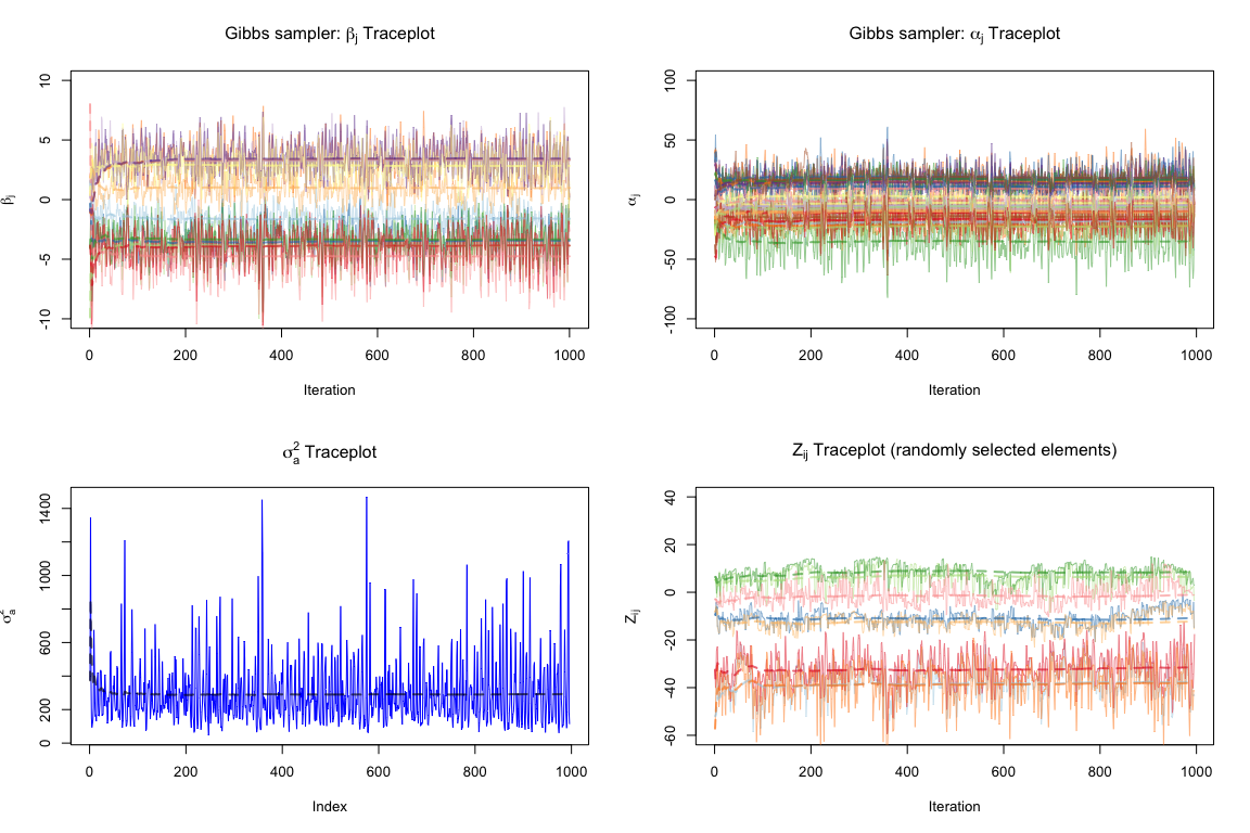
We see that our Gibbs sampler converges fairly fast and well, according to the traceplots above (we only use the first 5 iterations as burn-in); these traceplots reveal no signs of the chain being necessarily stuck anywhere at any point. Note that the \(\boldsymbol\beta\) components converge reasonably well, perhaps due to the initialization to reasonable OLS estimates. Also note that we are implicitly also modeling shrinkage through the prior on \(\beta_j\), assumed to be centered at 0, and this (along with the fact that our features are scaled) explains why the \(\beta_j\) components are centered about 0.

For robustness, we can also plot Autocorrelation function (ACF) plots for the \(\beta_k\) and \(\alpha_i\) components. ACF plots display the autocorrelation between samples in our chain as a function of the lag (number of steps separating the samples). A well-mixed chain will have low autocorrelations for small lags, indicating that the samples are relatively independent and the chain is exploring the parameter space efficiently. We select 5 components from each to evaluate at random.

par(mfrow = c(5,2), mar=c(2,2,3,2)) 
set.seed(220)
for(i in 1:5){
    kcomp = sample(1:p, 1)
    icomp = sample(1:N, 1)
    acf(track_beta[,kcomp], lag.max = 1000, main=paste0('Gibbs: beta_',kcomp))
    acf(track_alpha[,icomp], lag.max = 1000, main=paste0('Gibbs: alpha_',icomp))
}

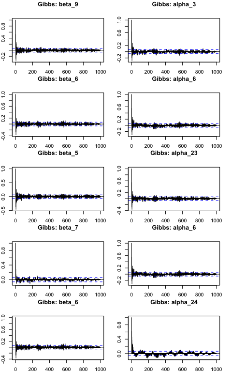
The ACF plots above display proper mixing in the chain as the autocorrelation drops rapidly toward 0 when lag increases, suggesting efficient posterior estimates. Further, the ACF plots are similar across the chains, suggesting that the mixing and convergence properties are consistent.

Part 6

We want to summarize our posterior inference results. We can first provide posterior summaries of each \(\beta_k\) (for the $k$-th covariate). Again, note that we scaled the feature matrix, which will affect our values for \(\beta_k\); however, this simply means we can make standardized predictions using our model (or unstandardize \(\mathbf X\) by multiplying by variance and adding mean back). For stability, we consider the last half of the chain when making posterior summaries.

Mean = apply(track_beta[500:nrun,], 2, mean)
beta_quantiles = apply(track_beta[500:nrun,], 2, function(x) quantile(x, c(0.025, 0.5, 0.975)))
beta_post = t(rbind(Mean, beta_quantiles)) %>% as.data.frame
colnames(beta_post) = c('mean', 'p025', 'median', 'p975')
beta_post$stat = colnames(X)

library(ggplot2)
ggplot() + 
    geom_point(data = beta_post, aes(x = stat, y = mean), 
                color = 'blue', alpha = 0.5) + 
    geom_point(data = beta_post, aes(x = stat, y = median), 
                color = 'green', alpha = 0.5) + 
    geom_errorbar(data = beta_post, aes(x = stat, y = median, ymin=p025, ymax=p975), 
                width = 0.1) + 
    geom_hline(yintercept = 0, linetype = 'dashed', color = 'gray70') + 
    theme_minimal() + 
    xlab('Player statistic') + ylab('Posterior Estimate')

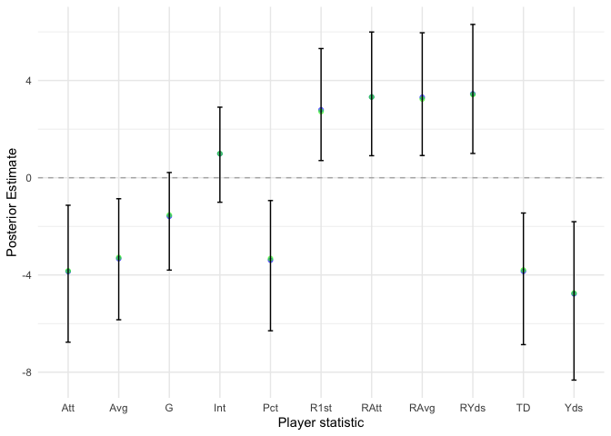
Our results about the \(\beta_k\) components are very reassuring. The 95% posterior intervals and directions make intuitive sense. For example, the estimate for the touchdown percentage of a player is significantly less than 0, which makes sense as touchdown percentage would generally increase the latent score of a player, thereby decreasing their rank.

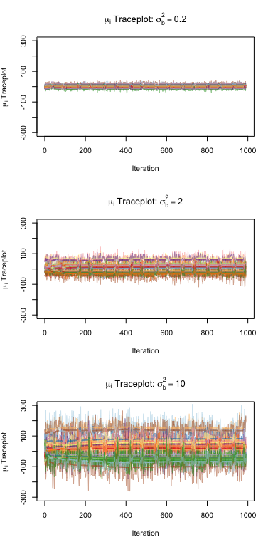
Under this model, we also have that the true score for player \(i\) is simply \(\mu_i = \alpha_i + \mathbf x_i^\top \boldsymbol\beta\). We can find the posterior mean of each player’s score, namely \(\hat\mu_i = \mathbb E[\alpha_i + \mathbf x_i^\top \boldsymbol\beta\\|\boldsymbol\tau]\). We try this at different values of \(\sigma^2_b\) to evaluate how our results are affected. Below, we consider the traceplot of this posterior mean for each \(\sigma^2_b \in \{0.2, 2, 10\}\) to evaluate the stability of our estimates, and we report the posterior means for each player’s score. Note that ranking based on this score is invariant of score scaling.

sig2_bs = c(0.2, 2, 10)
postMeans = list()

par(mfrow = c(3,1))
for(sig2_b in sig2_bs){
    gibbs_res = run_Gibbs(nrun=nrun, nu_a=1, s2_a=0.5, sig2_b=sig2_b, X=scale(X), origRank=t1)
    track_mu = -t(t(gibbs_res[[2]]) + X %*% t(gibbs_res[[1]]))
    postMeans[[as.character(sig2_b)]] = scale(apply(track_mu[500:nrun,], 2, mean))
    
    plot_trace(track_mu[10:nrun,], ylim = c(-300, 300), 
                label = expression(mu[i]*' Traceplot'))
    title(bquote(paste(mu[i], ' Traceplot: ', sigma[b]^2 == .(sig2_b))))
}

Below, we have the posterior means for each player’s scores, standardized within run, since ranking is invariant of score ranking.

scores_sig2_b = matrix(0, nrow = N, ncol = 3)
colnames(scores_sig2_b) = paste0('sig2b=', sig2_bs)
rownames(scores_sig2_b) = rownames(t1)

for(j in 1:length(sig2_bs)){
    res = postMeans[[as.character(sig2_bs[j])]]
    for(i in 1:N) scores_sig2_b[i,j] = res[rownames(res) == rownames(t1)[i],1]
}
scores_sig2_b

##                     sig2b=0.2     sig2b=2    sig2b=10
## Andrew Luck        1.89708772  2.01058105  1.98251462
## Aaron Rodgers      0.56490874  0.51471910  0.55479801
## Peyton Manning     1.73736171  1.78489779  1.77879573
## Tom Brady          1.65630310  1.74072182  1.76683076
## Tony Romo          1.01231107  0.97952461  1.04549961
## Drew Brees         0.37691179  0.36625193  0.38027823
## Ben Roethlisberg   0.83564834  0.76861660  0.81145085
## Ryan Tannehill     0.36673456  0.30498502  0.29618567
## Matthew Stafford   0.31665262  0.29388618  0.28134439
## Mark Sanchez       0.14644438  0.15259991  0.09271523
## Russell Wilson    -0.65861862 -0.70439581 -0.76113658
## Philip Rivers      0.03483141  0.01518099 -0.03470465
## Cam Newton        -0.41038472 -0.46796831 -0.52909854
## Eli Manning       -0.99173003 -0.90467347 -0.90922537
## Matt Ryan         -0.74266520 -0.69863887 -0.70611211
## Andy Dalton       -0.82945836 -0.85680412 -0.86903818
## Alex Smith        -0.75495806 -0.77510834 -0.77429229
## Colin Kaepernick  -0.81721675 -0.83430930 -0.86243836
## Joe Flacco         0.33782443  0.31985761  0.28309821
## Jay Culter         0.79739071  0.70301087  0.72569667
## Josh McCown       -0.80295215 -0.84824725 -0.82180304
## Drew Stanton      -1.70759987 -1.68088790 -1.60454467
## Teddy Bridgewater -1.06465500 -1.01853670 -1.03402365
## Brian Hoyer       -1.30017181 -1.16526341 -1.09279054

We see that as \(\sigma^2_b\) increases, the variance among the \(\mu_i\) scores increase greatly as seen in the traceplots; however, the ranking of the players does not necessarily change too much. This makes sense, again, given the invariance of rank to score scaling.

We can also report posterior probabilities for Tom Brady’s true score \(\mu_4\) to be better (namely lower, thereby leading to a better “lower” rank) than each of the proceeding quarterbacks (e.g. Manning, Rodgers, and Luck). We assume \(\sigma^2_b = 0.5\) again.

gibbs_res = run_Gibbs(nrun=nrun, nu_a=1, s2_a=0.5, sig2_b=sig2_b, X=scale(X), origRank=t1)
track_mu = t( t(gibbs_res[[2]]) + X %*% t(gibbs_res[[1]]) )
probs = apply(sapply(1:3, function(i) 
    apply(track_mu, 1, function(x) x[4] > x[i])), 2, mean)
cat(paste0(colnames(track_mu)[1:3], ": ", probs, '\n'))

## Andrew Luck: 0.644
## Aaron Rodgers: 0.021
## Peyton Manning: 0.559

These probabilities make great sense given the rankings in Table 1 (for example, Brady is almost consistently ranked lower Rodgers); however, we see the covariate adjustment in play here as well. For example, even though Andrew luck receives almost consistently better ranks than Brady, based on our posterior scores, Brady has a 64.4% probability of still being ranked better. We can provide an overall approximate 90% credible interval for each entity’s aggregated ranking, based on the estimated scores \(\hat\mu_i\).

rank_post = t(apply(apply(track_mu[10:nrun,], 1, function(x) rank(x)), 1, 
                    function(x) quantile(x, c(0.05, 0.5, 0.95))))
colnames(rank_post) = c('p5', 'median', 'p95')
rank_post = data.frame(rank_post)
rank_post$player = rownames(rank_post)
rank_post$player = factor(rank_post$player, levels = rank_post$player[order(rank_post$median)])

ggplot() + 
    geom_errorbar(data = rank_post, aes(x = player, y = median, ymin=p5, ymax=p95), 
                width = 0.15) + 
    geom_point(data = rank_post, aes(x = player, y = median), 
                color = 'red', alpha = 1) + 
    theme_minimal() + 
    xlab('Player') + ylab('Posterior Rank') + 
    theme(axis.text.x = element_text(angle = 45, hjust = 1, vjust = 1))

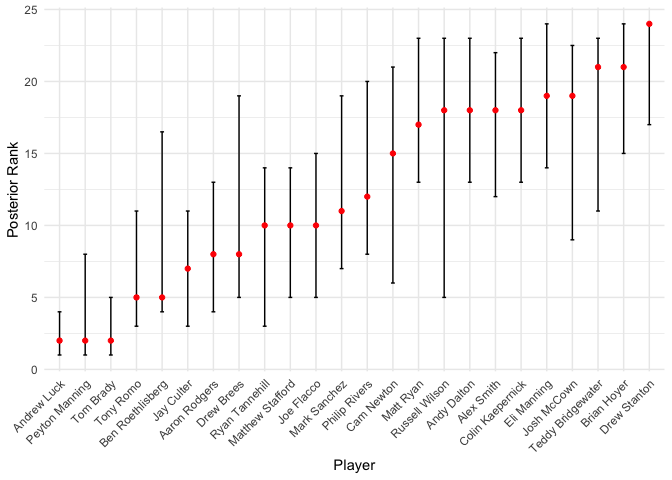
These rankings seem pretty good, relative to the rankings in Table 1!

Part 7

Comment on how well the current model fits the data. In particular, is there any evidence that some rankers may not be as good as others and may use the covariates differently? Report any model weaknesses you can find and make suggestions on how you might revise your model.

The model here fits the data reasonably well, as the rankings do in fact match those in Table 1, even while accounting for covariates. To assess whether there is any evidence that some rankers may not be as good as others and may use the covariates differently, we can consider the traceplots of scores for two different rankers, ranker 1 and ranker 2.

par(mfrow = c(1,2))
set.seed(220)
plot_trace(t(track_Z[,1,])[10:nrun,], ylim = c(-60, 40), 
            label = expression(Z[i1]))
title(expression(Z[i1]*' Traceplot (ranker 1)'))
set.seed(220)
plot_trace(t(track_Z[,10,])[10:nrun,], ylim = c(-60, 40), 
            label = expression(Z[ij]))
title(expression(Z[i2]*' Traceplot (ranker 2)'))

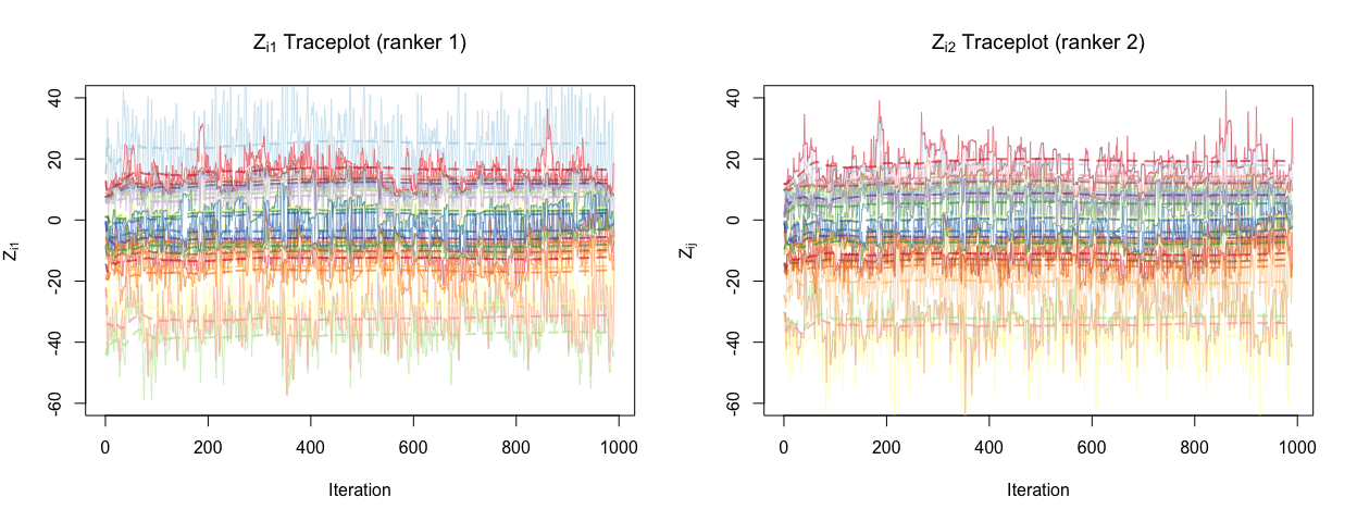
We do see some discrepancy between these two rankers, suggesting that rankers and in fact using covariates differently to construct their scores, since the player random effect takes on the same value across the rankers. Further, it makes sense that we have ranker discrepancy since we adopt a hierarchical approach to this problem, and this is clearly illustrated by the graphical model from Part 2.

We can propose a few extensions or suggestions to revise this model. We can potentially add interactions terms between rankers and covariates in the model; this will allow the model to capture different relationships between the covariates and the response for different rankers, thereby accounting for potentially bad rankers. We can also explore how rankers may be using covariates differently by using our hierarchical modeling approach. Further, we can perform something similar to a “subgroup analysis”, where, if we know (a priori) that there are different groups of rankers (perhaps some are biased toward different conferences, for example), we perform separate analyses for each group to investigate potential differences in the relationships between the covariates and the response.

Finally, we adopted a Normal prior on the feature coefficients \(\boldsymbol\beta\), which is equivalent to Ridge regularization. Perhaps we can explore other shrinkage mechanisms, such as LASSO for example, which has the advantage of typically shrinking some coefficients to exactly 0. If we believe that some covariates are simply noise and not useful for ranking, then LASSO might be useful in that context.