Statistical Optimization Techniques

Central to solving many scientific and machine learning problems is optimization. Excluding a handful specifically-structured problems, we typically have no guarantee of finding global optima; instead, we settle for reasonable good local modal solutions. Thus, optimization has largely taken the form of mode finding. Further, note that typically, mode finding of some target function is equivalent to root finding for its gradient, if it exists.

Overflow and Underflow

Developing robust strategies to deal with underflow and overflow is often of critical importance to many optimization problems. For example, in the context of statistical inference, we may want to maximize the likelihood function to derive the maximum likelihood estimator (MLE); however, especially with larger samples sizes, directly computing the likelihood can often lead to overflow or underflow. We typically never want to multiple many probabilities or density values directly. Instead, we can operate on the logarithmic scale when possible. When computing the summation or product of many small or large numbers, it is better to do this properly on the logarithmic scale.

Take the following problem for an example of dealing with underflow in particular. Let us say we have a potentially biased coin whose probability of showing head is \(\theta\), and a priori we know \(\theta\) is either 0.5 or 0.6, with equal probabilities. We toss the coin \(n=10,000\) times and observe \(x=5,510\) heads. Our goal then is to compute the posterior probability \(\Pr(\theta = 0.6 \\| n, x)\).

We can first find a simplified expression for this posterior probability of interest using Bayes Theorem and LOTP (note, \(n\) is known, but we include it in the expression below for clarity),

We can see from the expression above that we are in fact working with some very small probabilities; \(0.6^{5510}\) evaluates directly to 0 in R due to underflow. To avoid such underflow errors, we can instead work with log-posterior probabilities,

where \(a =\max\{\left(x\log 0.6 + (n-x)\log 0.4\right) , n\log0.5\}\). Note that above, we are implementing the LogSumExp function (also known as the “SoftMax trick”) to compute the log of the denominator (which is the log of summed exponentiated log terms). This is a simple idea which essentially involves subtracting the maximum, \(a\), from each exponentiated term, thereby reducing underflow errors.

With these robust strategies defined for dealing with underflow, we can now implement our ideas below to compute the posterior probabilities of interest.

compute_posterior <- function(n, x, return_val=F, verbose=T){
  log_numer = x*log(0.6) + (n-x)*log(0.4)
  a = max(log_numer, n*log(0.5))
  log_denom = a + log(exp(log_numer - a) + exp(n*log(0.5) - a))
  log_posterior = log_numer - log_denom
  
  if(verbose){
    cat(paste0('log-posterior prob: ', log_posterior,'\n'))
    cat(paste0('    posterior prob: ', exp(log_posterior),'\n'))
  }
  
  if(return_val) return(log_posterior)
}
compute_posterior(10000, 5510)

## log-posterior prob: -0.0664927009465828
##     posterior prob: 0.935669745334858

We find that the posterior probability that \(\theta = 0.6\) is roughly 0.94. For fun, we can evaluate how this posterior probability varies depending on the number of heads we observe out of \(n\) coin flip trials.

ns = c(25, 50, 100, 1000, 10000)
head_prop = seq(0, 1, 0.001)
probs_df = data.frame(n = rep(ns, each = length(head_prop)), 
                      heads = rep(head_prop, length(ns)), 
                      log_post_probs = 0)
probs_df$heads_obs = probs_df$heads * probs_df$n
probs_df = probs_df[round(probs_df$heads_obs) == probs_df$heads_obs,]

for(n in ns){
  start_idx = which(probs_df$n == n)[1]
  idxs = start_idx:(start_idx + sum(probs_df$n == n)-1)
  obs_heads = probs_df$heads_obs[idxs]
  lpost_probs = lapply(obs_heads, function(x) 
    compute_posterior(n, x, return_val=TRUE, verbose = FALSE)) %>% unlist
  probs_df$log_post_probs[idxs] = lpost_probs
}

ggplot(probs_df, aes(x=heads, y = exp(log_post_probs), color = as.factor(n))) +
  geom_line(size = 2, alpha = 0.8) + 
  ylab('Posterior probability theta = 0.6') + 
  xlab('Proportion of heads observed') + 
  geom_vline(xintercept = 0.55, color = 'gray20', linetype = 'dashed') + 
  guides(color = guide_legend('Number of \nCoin Flips (n)'))

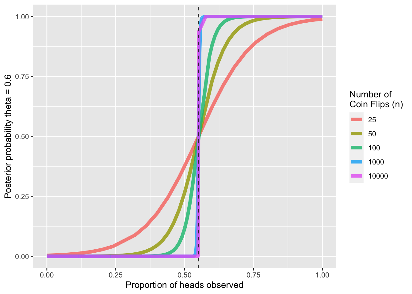
As expected, we see that as the proportion of heads increases, the posterior probability that \(\theta = 0.6\) increases, with an inflection point at \(\theta = 0.55\). Further, with larger sample sizes, the increase in posterior probability past \(0.5\) increases more sharply; at larger samples sizes, we are more sure in our inference for a given porportion of heads observed.

Such computations would not be possible without robust strategies for dealing with underflow. Now, back to our discussion of optimization.

Simulating Data for Optimization

Throughout our discussion of different optimization techniques, we can use the probit regression model as a motivating example. We can simulate data from this model and apply various optimization algorithms to this data for the sake of comparison.

The probit regression model assumes the following relationship between a binary response \(y_i\) and a \(p\)-dimensional covariate vector \(\mathbf x_i\):

where \(\boldsymbol \beta = (\beta_1, \dots, \beta_p)^\top\) is an unknown \(p\)-dimensional vector of coefficients, and \(\Phi\) is the CDF of the standard Normal. Suppose we observe the \((y_i,\mathbf x_i)\)’s and are interested in estimating \(\boldsymbol\beta\).

We can simulate \(\mathbf{x}_i'\overset{iid}\sim \mathcal{N}(0,2\mathbb{I}_p)\) for \(i = 1,\dots,n\) with \(n=300\). Note that to do this, we can simulate each individual component of \(\mathbf{x}_i\) independently. Then, we can construct a coefficients vector \(\boldsymbol{\beta}\) as follows: \(\beta_j = 1\) if \(j\) is odd and -1 otherwise, for \(j = 1,\dots,p\). We take this \(\boldsymbol\beta\) to be the “true” underlying coefficient vector that we try to estimate using a variety of optimization techniques. Finally, we can use \(\mathbf{x}_i\) and \(\boldsymbol{\beta}\) to simulate \(y_i\). We can simulate data for both \(p = 1\) (one-dimensional) and \(p = 10\) (multi-dimensional).

n = 300
sim_probit <- function(p){
    x = sapply(1:p, function(x) rnorm(n=n, mean=0, sd=sqrt(2)))
    beta = as.matrix(ifelse(1:p %% 2 == 0, yes = -1, no = 1))
    y = pnorm(x %*% beta)
    return(list(x, beta, y))
}

# Try p=1 and p=10
set.seed(221)
sim_p1 = sim_probit(p=1)
sim_p10 = sim_probit(p=10)

With our data simulated, the goal is now to find the optimal underlying \(\boldsymbol\beta\) that generated our simulated data (which we pretend that we do not know). We can take a likelihood-based approach to finding the optimal underlying \(\boldsymbol\beta\).

Evaluating the Log-Likelihood

First, we will need to write a robust subroutine to evaluate the log-likelihood function of \(\boldsymbol\beta\), which can be simplified by taking advantage of some useful properties of logarithms,

Note that in the log-likelihood simplification above, we evaluate the term \(\left(1 - \Phi(\mathbf{x}_i^\top\boldsymbol{\beta})\right)\) as \(\Phi(-\mathbf{x}_i^\top\boldsymbol{\beta})\) by the symmetry of the Normal CDF. This is advantageous here as it avoid numerical imprecision errors if \(\Phi(\mathbf{x}_i^\top\boldsymbol{\beta})\) returns a value too close to 1 (specifically greater than 0.9999999 in R); in such cases R would simply evaluate \(\left(1 - \Phi(\mathbf{x}_i^\top\boldsymbol{\beta})\right)\) as 0, which will return \(-\text{Inf}\) when we subsequently take the logarithm.

We can now implement this into a subroutine to evaluate the log-likelihood below.

eval_logLik <- function(x, beta, y) {
  cdf_vals = pnorm(x %*% beta)
  ncdf_vals = pnorm(-x %*% beta)
  loglik_terms = y*log(cdf_vals) + (1-y)*log(ncdf_vals)
  return(sum(loglik_terms))
}

Evaluating the Gradient of the Log-Likelihood

As mentioned in the Introduction earlier, typically, mode finding of some target function (the log-likelihood in this case) is equivalent to root finding for its gradient. We can thus write a subroutine to evaluate the gradient of the log-likelihood function. This will prove useful for some optimization techniques we discuss next. First, we solve for this gradient mathematically.

We can now implement this into a subroutine below.

eval_grad_logLik <- function(x, beta, y) {
  cdf_vals = pnorm(x %*% beta)
  ncdf_vals = pnorm(-x %*% beta)
  pdf_vals = dnorm(x %*% beta)
  
  scalars = y*pdf_vals/cdf_vals + (y-1)*pdf_vals/(ncdf_vals)
  gradient = t(t(scalars) %*% x)
  
  return(gradient)
}

With all of this defined, we can finally discuss the first optimization, or more specifically root finding, method: Bisection.

Bisection Method

Perhaps the simplest of all root finding methods for a 1-dimensional continuous function \(f(x)\) is the bisection method. The algorithm proceeds as follows:

• Initialize by finding two numbers \(a < b\) such that \(f(a) \cdot f(b) < 0\), and set \(\ell = a\) and \(u = a\).
• Then, bisect by letting \(c = (\ell + u)/2\) and computing \(f(c)\). If it is sufficiently close to 0, terminate. Otherwise set \(u \leftarrow c\) if \(f(\ell) \cdot f(c) < 0\) and \(\ell \leftarrow c\) if \(f(\ell) \cdot f(c) > 0\).

This algorithm converges fairly quickly, as the “error”, or distance from the root, is essentially cut in half with each iteration. Again, if we seek to find optima for a differentiable function \(g(x)\), we can find the root of its derivative \(g′(x)\), requiring only knowledge of the initialization parameters \(a,b\) that bound a local optima.

Returning to out probit regression model, for \(p=1\), we can write a bisection algorithm to find the MLE \(\hat\beta_{MLE}\). We seek to find a root of the gradient of the log-likelihood, which is equivalent to finding the maximum of the log-likelihood since the log-likelihood of a probit regression is globally concave.

Let \(f(x)\) denote the gradient of the log-likelihood evaluated at \(\beta = x\). Our implementation below first takes in two numbers \(a < b\) such that \(f(a)f(b) < 0\) (otherwise an error is returned). The bisection algorithm then proceeds as described earlier. A plotting parameter is also included to visualize the convergence of the bisection algorithm.

bisection_find <- function(fx, epsilon, initials, x, y, plotting=TRUE) {
  l = min(initials); u = max(initials)
  if(fx(x=x, beta=l, y=y) * fx(x=x, beta=u, y=y) >= 0) {
    return("ERROR: Initial values provided do not evaluate to have opposite signs. 
           Select different values.\n")
  }
  
  # First iteration:
  iter = 1
  cx = (l + u)/2
  fc = fx(x=x, beta=cx, y=y)
  c_rec = c(cx)
  fc_rec = c(fc)
  
  while(abs(fc) > epsilon){
    if(fx(x=x, beta=l, y=y) * fc < 0) u = cx
    if(fx(x=x, beta=l, y=y) * fc > 0) l = cx
    cx = (l + u)/2
    fc = fx(x=x, beta=cx, y=y)
    
    c_rec = c(c_rec, cx)
    fc_rec = c(fc_rec, fc)
    iter = iter + 1
  }
  cat(paste0('Converged in ', iter,' iterations.\nRoot found at ', cx, '.\n'))
  
  if(plotting==FALSE) return(cx)
  
  range_vals = seq(min(initials), max(initials), 0.001)
  rec = c()
  for(i in range_vals) rec = c(rec, fx(x=x, i, y=y))
  plot(range_vals, rec, type = 'l', xlab = 'Range of values, beta', 
       ylab = 'f(beta): Gradient of log-likelihood', 
       main = paste0('Bisection Algorithm Steps (converged in ', iter,' iterations)'))
  lines(c(min(initials), max(initials)), y = c(0,0), 
        type = 'l', col = 'red', lty = 'dashed', lwd = 1.75)
  points(c_rec, fc_rec, pch = 'x', col = 'navy')
  return(cx)
}

# Example below
x = sim_p1[[1]]; beta = sim_p1[[2]]; y = sim_p1[[3]]
root = bisection_find(fx = eval_grad_logLik, epsilon = 0.0001, initials = c(-5, 5), 
                      x=x, y=y, plotting=TRUE)

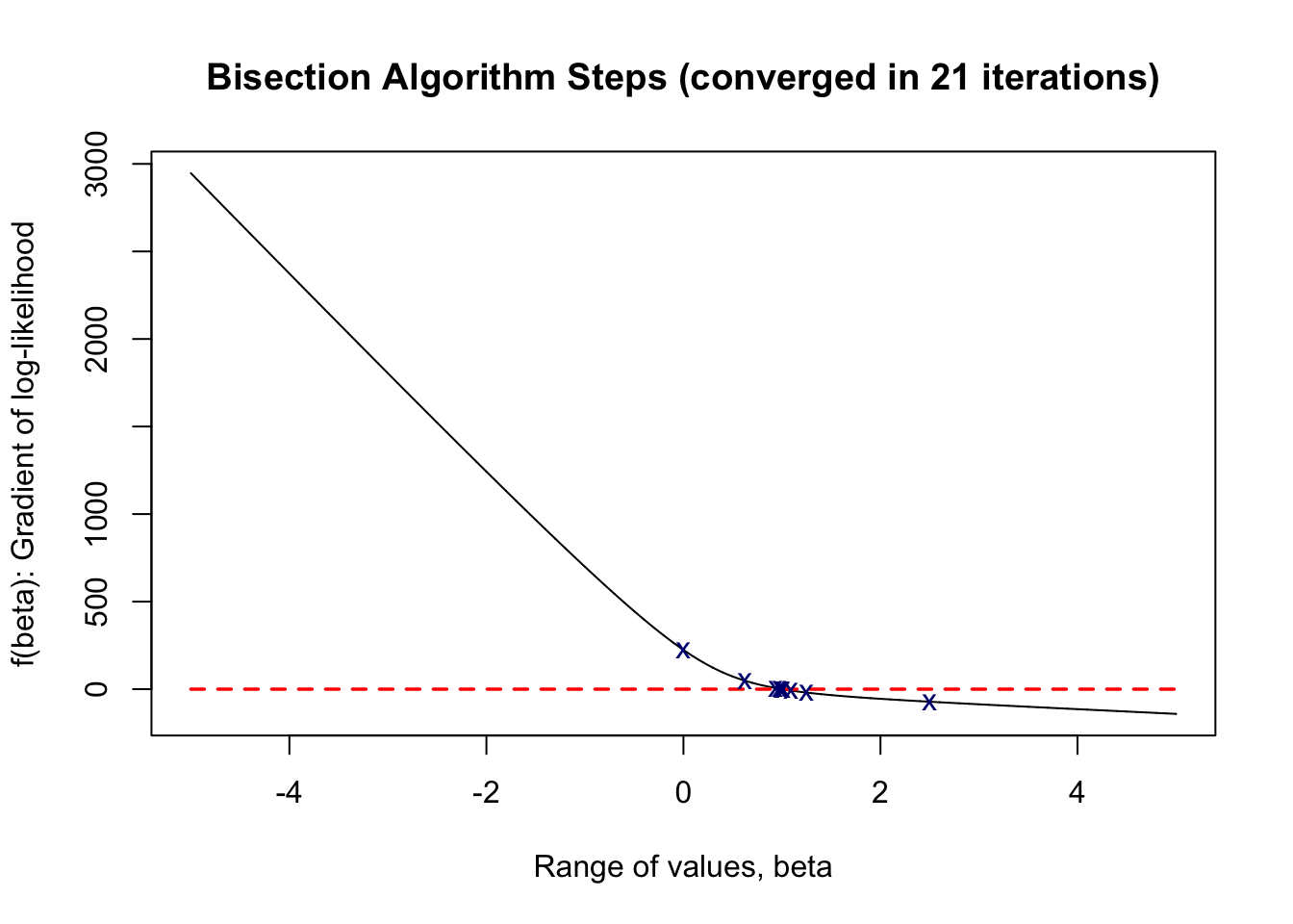
As shown above, our bisection algorithm converged in 22 iterations, finding a root at 0.99999952, which is very close to the true parameter value of \(\beta = 1\) in the 1-dimensional case.

We now turn to gradient-ascend algorithms to find the MLE of \(\boldsymbol\beta\) for the general \(p\)-dimensional case.

Gradient-based optimization methods